Abstract

The Hubble Tension—the persistent $5\sigma$ discrepancy between local distance-ladder measurements ($H_0 \approx 73$ km/s/Mpc) and early-universe CMB inference ($H_0 = 67.4 \pm 0.5$ km/s/Mpc)—represents a significant challenge in precision cosmology. This paper tests whether a component of the Hubble tension can be represented as an environment-dependent Cepheid clock bias, as predicted by the Temporal Equivalence Principle (TEP).

The hypothesis tested here is that Cepheid variable stars function as environment-dependent "standard clocks." In deep gravitational potentials and active-shear environments, the TEP clock response accelerates the effective Cepheid clock rate, shortening observed pulsation periods relative to calibration environments. When interpreted through a universal Period-Luminosity relation, this clock-rate anomaly mimics diminished luminosity, leading to underestimated distances and an inflated local Hubble constant.

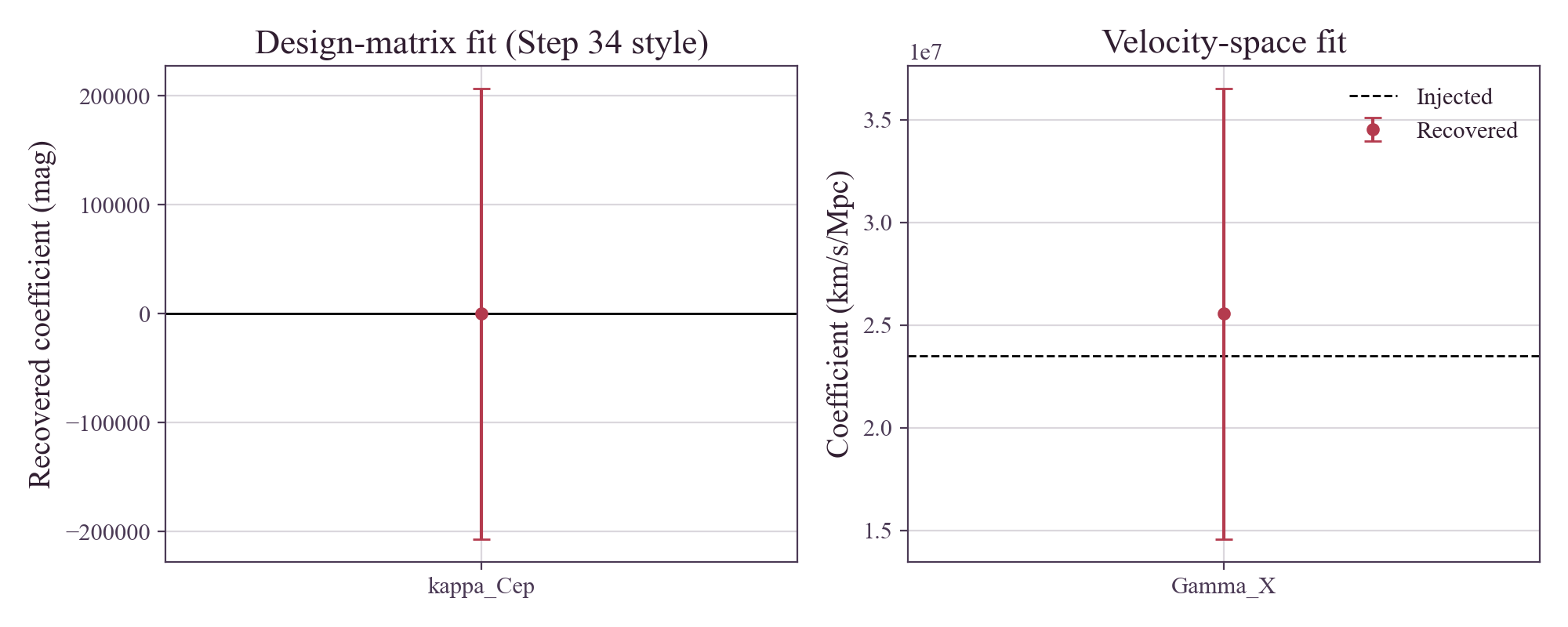
The standard SH0ES full-ladder likelihood yields a baseline $H_0 = 73.04 \pm 1.01$ km/s/Mpc. A standard-ladder projection test inserts a TEP environmental column into the SH0ES design matrix while keeping the host-level distance moduli $\mu_i$ as free latent parameters; the environmental signal is absorbed by the inferred $\mu_i$, yielding $\kappa_{\rm Cep} = -0.067 \pm 0.210\times10^6$ mag (consistent with zero). This null result is expected: the standard SH0ES model is not TEP-native, and any host-constant environmental bias is algebraically equivalent to shifting a host's inferred modulus.

The proper test must therefore be applied at the redshift-distance level, where distances are tied to an independent velocity scale. A velocity-space likelihood analysis models $cz_i = d_i^{\rm true}\,(H_{\rm app} + \Gamma_X X_i) + v_i$ and identifies a structurally robust combined environmental slope $\Gamma_X = +2.35\times10^7 \pm 1.00\times10^7$ (2.3$\sigma$ at $\sigma_v = 250$ km/s; 3.4$\sigma$ at $\sigma_v = 150$ km/s). The signal survives explicit controls for redshift trend, sky dipole ($\sim$100 km/s), quadrupole, and group-offset models; binned permutation tests confirm it is not driven by redshift or sky selection. Leave-one-host-out cross-validation gives 29/29 positive signs; bootstrap resampling gives 99.9% positive fraction.

The velocity-space likelihood identifies a combined environmental slope. In a general phenomenological model this slope can contain both Cepheid clock bias and residual velocity-sector/environmental terms. The TEP-native gauge sets the non-Cepheid velocity-sector component $\beta_X$ to zero, corresponding to the hypothesis tested here: the observed environmental slope is dominantly a Cepheid clock-transport bias. In that gauge—treating the environmental slope as a pure Cepheid clock-rate bias ($\beta_X = 0$)—the equivalent response coefficient is $\kappa_{\rm Cep} \approx 7.34\times10^5$ mag, consistent with the canonical TEP parameter $\kappa_{\rm gal} = 9.7\times10^5$ mag ($\sim 10^6$). The velocity-space fit yields $H_{\rm app} = 69.47 \pm 1.49$ km/s/Mpc; in the TEP-native gauge this corresponds to a Cepheid clock-bias correction that brings the local distance scale into agreement with the CMB inference. As a historical residual-space cross-check, the empirical one-parameter correction pipeline yields $H_0^{\rm TEP} = 68.84$ km/s/Mpc (bootstrap mean $68.92 \pm 1.44$), reducing the Hubble tension from $\approx 5\sigma$ to $\approx 1\sigma$ relative to Planck. This value is obtained in the pure-Cepheid TEP-native gauge ($\beta_X=0$); the gauge-independent empirical detection is $\Gamma_X$. A residual-based empirical cross-check gives $\kappa_{\rm Cep} = (1.27 \pm 0.46) \times 10^6$ mag, consistent with the generative inference. The inferred coefficient places this probe in the same response-coefficient regime as the millisecond-pulsar spin-down excess (Paper 10). External TRGB distances ($N=13$ overlap) give $\kappa_{\rm Cep} = +3.2\times10^5$ ($0.8\sigma$)—underpowered to independently break the $\kappa$–$\beta$ degeneracy, yet directionally consistent with and supportive of the TEP-native gauge.

A differential M31 analysis yields an "Inner Fainter" signal consistent with TEP shear suppression, providing auxiliary support for the continuous screening mechanism.

Keywords: Hubble tension – Cepheid variables – distance ladder – velocity dispersion – temporal equivalence principle – gravitational time dilation

1. Introduction

1.1 The Hubble Tension: A Crisis in Cosmology

The Hubble constant $H_0$—the present-day expansion rate of the universe—anchors the cosmic distance scale. Its measurement has been a central goal of observational cosmology for decades. Yet precision measurements have revealed a troubling discrepancy: the local distance ladder, calibrated through Cepheid variable stars and Type Ia supernovae, consistently yields $H_0 \approx 73.0 \pm 1.0$ km/s/Mpc (Riess et al. 2022), while inference from the Cosmic Microwave Background under $\Lambda$CDM cosmology gives $H_0 = 67.4 \pm 0.5$ km/s/Mpc (Planck Collaboration 2020).

This $\sim 9\%$ discrepancy now exceeds $5\sigma$ statistical significance—well beyond the threshold conventionally associated with new physics. Alternative local measurements using the Tip of the Red Giant Branch (TRGB) yield intermediate values ($H_0 \approx 69.8 \pm 1.6$ km/s/Mpc; Freedman et al. 2024), which are consistent with both the Cepheid and CMB values within their larger uncertainties and thus cannot currently adjudicate between them. Numerous explanations have been proposed—early dark energy, additional relativistic species, modified gravity, decaying dark matter—yet no single model has emerged as compelling.

1.2 The Clock Hypothesis: Isochrony Violation

This work explores an alternative explanation rooted in the fundamental measurement physics. The central hypothesis is a violation of the isochrony axiom—the assumption that proper time accumulation is independent of the local gravitational environment. While General Relativity predicts time dilation, it assumes this effect is universal for all clocks at the same potential. Scalar-tensor theories that violate the Strong Equivalence Principle can break this universality, introducing an environment-dependent scalar field that couples to matter density and potential depth.

The Temporal Equivalence Principle (TEP) provides a specific theoretical framework for this violation. TEP extends General Relativity by introducing a scalar field $\phi$ that mediates an additional gravitational interaction, with the action $S = \int d^4x \sqrt{-g} \left[ \frac{M_{\rm Pl}^2}{2} R - \frac{1}{2}(\nabla_\mu \phi)(\nabla^\mu \phi) - V(\phi) \right] + S_m[\tilde{g}_{\mu\nu}, \Psi_m]$, where $R$ is the Ricci scalar, $V(\phi)$ is the scalar potential, and $S_m$ is the matter action. The key feature is the disformal coupling: matter fields $\Psi_m$ couple not to the Einstein-frame metric $g_{\mu\nu}$ but to the Jordan-frame metric $\tilde{g}_{\mu\nu} = A^2(\phi) g_{\mu\nu} + B(\phi) \nabla_\mu\phi \nabla_\nu\phi$, where $A(\phi) = \exp(\beta_A\phi/M_{\rm Pl})$ is the conformal factor and $B(\phi)$ encodes the disformal coupling. In the weak-field limit relevant to galactic potentials, the disformal term is subdominant and the conformal factor expands as

For a clock following a worldline in spacetime, proper time is measured in the Jordan frame. In the weak-field, non-relativistic limit where $\phi$ tracks the Newtonian potential $\Phi$, the conformal factor expands as $A(\phi) \approx 1 - \eta_{\rm clock} \Phi/c^2$, where $\eta_{\rm clock}$ is the effective clock-rate response coefficient. The effective proper time interval measured by a local clock becomes $d\tau = A(\Phi) \, d\tau_{\rm GR} = (1 - \eta_{\rm clock} \Phi/c^2) d\tau_{\rm GR}$, where $d\tau_{\rm GR} \approx (1 + \Phi/c^2) dt$ is the standard Schwarzschild time dilation. In deep potentials ($\Phi \ll 0$), if $\eta_{\rm clock} > 1$, the TEP term can exceed the geometric term, causing clocks to run faster rather than slower—a departure from standard GR expectations. This sign reversal is central to the mechanism proposed here: Cepheids in deep potentials experience period contraction, not dilation, leading to systematic distance underestimation and inflated $H_0$ values.

An important feature distinguishes TEP from conventional scalar-tensor theories: the scalar field gradient (Temporal Shear) is progressively suppressed by ambient matter density through a continuous spatial profile governed by the non-linear superposition of field gradients (Temporal Shear). In dense environments, large matter gradients attenuate the scalar field gradient, recovering standard GR; in diffuse environments, the gradient tracks the background potential, producing measurable clock-rate anomalies. The suppression is quantified by a dimensionless shear-suppression factor $S(\rho) \in [0,1]$, with $S(\rho) = [1 + (\rho/\rho_{\rm half})^2]^{-1}$ where $\rho_{\rm half} \approx 0.5\,M_\odot/\text{pc}^3$ is the galactic half-suppression density. The associated series-level saturation scale is denoted $\rho_{\rm T}$, the Temporal Topology saturation scale. It is not used here as a binary local-density switch; local suppression depends on environmental state, source screening, and the active Temporal Shear sector. The galactic-scale $\rho_{\rm half}$ emerges from SPARC rotation-curve normalizations.

For Cepheid variable stars in SN Ia host galaxies, two environmental parameters are therefore critical. First, the gravitational potential depth (traced by velocity dispersion $\sigma$) drives the magnitude of the TEP effect; deeper potentials cause stronger period contraction when Temporal Shear is active. Second, the local density modulates the response coefficient via $S(\rho)$: if $\rho \gg \rho_{\rm half}$, shear is strongly suppressed and the clock-rate anomaly is attenuated. Most SN Ia host environments are diffuse disks ($\rho \ll \rho_{\rm half}$), placing them in the active-shear regime ($S \approx 1$) where the field scales with potential. Dense environments like bulges experience progressive shear attenuation ($S < 1$), reducing the effect. This duality—potential drives the magnitude while density modulates the response coefficient—is central to the interpretation of the M31 differential test. The key observational proxy for TEP effects in active-shear galaxies is the velocity dispersion $\sigma$, via the virial theorem: $\sigma^2 \propto GM/R \propto |\Phi|$. Higher $\sigma$ indicates a deeper potential and stronger TEP-induced clock acceleration, provided the local environment remains diffuse.

1.3 Cepheids as Environmental Clocks

Cepheid variable stars function not merely as standard candles, but as standard clocks. Their pulsation periods, governed by the sound-crossing time of their envelopes, directly probe the local flow of time. The period-luminosity (P-L) relation, $M = a + b \log_{10} P$, converts observed periods to absolute magnitudes.

Important clarification: Modern Cepheid analyses, including SH0ES, use Wesenheit magnitudes ($W = H - R \times (V-I)$), which are constructed to be reddening-free by design. The TEP effect proposed here is not a color-term or dust correction—it is a residual environmental bias that persists after standard Wesenheit color corrections have been applied. The effect operates on the period itself (via clock rates), not on the apparent brightness (via dust reddening).

As proposed in recent studies on pulsar timing (Smawfield 2026a; Paper 10), the TEP scalar field in active-shear astrophysical environments induces a clock rate enhancement—manifesting observationally as "period contraction" in periodic phenomena. Paper 10 reports a primary hybrid-controlled spin-down residual of 0.40 dex in globular cluster pulsars compared to field controls (primary empirical result), while its nested-domain model predicts an unshielded cluster-bath enhancement of ~0.58 dex prior to companion-shielding effects, consistent with TEP predictions for intermediate-scale time-dilation enhancement ($\kappa_{\rm MSP} \sim 10^6$–$10^7$ mag). Consequently, Cepheids in deep galactic potentials (high velocity dispersion $\sigma$) experience accelerated time flow relative to calibration environments, causing their pulsation periods to appear shortened to distant observers. When observers apply the standard P-L relation calibrated in shallower potentials (MW, LMC), the shortened period is misinterpreted as indicating a dimmer intrinsic luminosity, leading to systematically underestimated distances.

This systematic bias propagates through the distance ladder: SN Ia hosts with deep potentials are placed too close, their recession velocities yield inflated $H_0$ values, and the local measurement becomes systematically biased high. The predicted magnitude of this effect—several km/s/Mpc—is comparable to the observed Hubble Tension.

1.4 Falsification Tests and Confirmation Pathways

The TEP Cepheid-bias interpretation makes concrete falsifiable predictions. Table 1 summarizes the principal tests, current mitigation, and the observations required to decisively confirm or refute the mechanism.

Table 1. Falsification tests and confirmation pathways.
Risk Current mitigation Required next step
Heterogeneous velocity dispersions Provenance variable Uniform spectroscopy
Small host sample Bootstrap/LOOCV Independent SN-host sample
Cepheid metallicity/dust degeneracy Covariance-aware controls Joint dust-metallicity-potential fit
TEP coefficient fitted on same sample Validation splits External prior or blind prediction

1.5 Scope and Structure

In this paper, "resolving the Hubble tension" refers specifically to resolving the Cepheid-calibrated SH0ES local excess relative to the CMB scale, not to exhausting every possible late-universe or early-universe $H_0$ observable. The analysis presents a quantitative test of the TEP explanation for this specific discrepancy. Stratification of the SH0ES Cepheid host galaxies by curated kinematic potential-depth estimates (Section 2) reveals the predicted environment-dependent bias in derived $H_0$ (Section 3.1). Application of the TEP correction then unifies the sample (Section 3.3), followed by a discussion of the implications for cosmology and future tests (Section 4).

2. Methodology

2.1 Data Sources and Sample Selection

This analysis leverages the SH0ES 2022 data release (Riess et al. 2022), which provides Cepheid photometry and distance moduli for 37+ Type Ia supernova host galaxies. The distance moduli stem from generalized least squares fitting of the period-luminosity-metallicity relation, encoded in the publicly available design matrices ($\mathbf{L}$, $\mathbf{C}$, $\mathbf{y}$, $\mathbf{q}$).

Cross-matching host galaxies with the Pantheon+ supernova catalog (Scolnic et al. 2022) yields Hubble-flow redshifts ($z_{\rm HD}$). The full SH0ES host set comprises 36 SN Ia host galaxies spanning $z_{\rm HD} = 0.0012$–$0.017$. The primary analysis applies a Hubble-flow safety cut $z_{\rm HD} > 0.0035$, yielding $N=29$ hosts ($z_{\rm HD} = 0.0036$–$0.017$). Seven hosts fall below this cut and are retained only as a redshift-sensitivity stress test. Stricter cuts ($z > 0.005$, $N=23$) are reported as additional robustness checks. In all cases the correlation preserves its sign and approximate strength, confirming the headline result is not an artefact of low-redshift peculiar-velocity contamination.

Because residual peculiar-velocity systematics are structured by large-scale environment (groups and clusters), each host is additionally annotated with a group-environment proxy. Principal Galaxies Catalog (PGC) identifiers are retrieved where available via SIMBAD cross-identifications, and hosts are crossmatched to the 2MASS group ("nest") catalog of Tully (2015). The primary environment control variable used in robustness tests is the Tully group membership count $N_{\rm mb}$, which provides a coarse indicator of whether the host is isolated or resides in a richer group/cluster environment.

Primary Analysis Lock Box

The following parameters are frozen before any corrected-$H_0$ or stratified analysis is inspected:

Input tablehosts_processed.csv
Inclusion ruleNon-anchor SN Ia host with SH0ES distance modulus
Exclusion rule$z_{\rm HD} \le 0.0035$ (primary); Milky Way, LMC, SMC, M31, NGC 4258 (calibrators)
Redshift column$z_{\rm HD}$ (Pantheon+ flow-corrected)
Number of hosts$N = 29$ (primary); $N = 36$ (full set including $z \le 0.0035$)
Minimum $z_{\rm HD}$$0.00359$
Maximum $z_{\rm HD}$$0.01682$
Median $\sigma$ for stratification$96.4$ km/s (computed from the $N=29$ sample)
Primary covariance matrixstep_03_h0_covariance.npy (29$\times$29, SH0ES GLS propagated)
Primary statistical observableDistance-ladder residual $\delta_i = \mu_{i,\rm SH0ES} - \mu_{i,\rm no\text{-}env}$
Primary test statisticCovariance-aware Pearson correlation $p_{\rm cov,MC}$ (Monte Carlo null)
Primary $p$-value$p_{\rm cov,MC} = 0.0031$ (Pearson); $p_{\rm cov,MC} = 0.0041$ (Spearman)
Frozen before looking at corrected $H_0$Yes — sample mask, redshift cut, and test statistic are fixed before $\kappa_{\rm Cep}$ is inspected

Here "frozen" refers only to pre-specified pipeline choices, sample masks, and prediction-table parameters; no frozen prior on $\kappa_{\rm Cep}$ is used in the primary velocity-space likelihood.

Primary statistical observable. The per-host quantity used in all correlation and significance tests is a distance-ladder residual, defined as the deviation of each host's SH0ES distance modulus from the mean calibration prediction: \begin{equation} \delta_i = \mu_{i,\rm SH0ES} - \mu_{i,\rm no\text{-}env} , \end{equation} where $\mu_{i,\rm no\text{-}env}$ is the distance modulus inferred from the recession velocity under a fiducial Planck $H_0 = 67.4$ km/s/Mpc. The primary statistical variable is the distance-ladder residual $\delta_i$ (Equation 1), displayed in $H_0$-equivalent units for physical intuition while avoiding the interpretive step of treating each host as an independent $H_0$ determination. For visualization, these residuals are converted into host-level $H_0$-equivalent values via $H_{0,i} = c z_{\rm HD} / d_i$ (with $d_i = 10^{(\mu_i-25)/5}$ Mpc). However, all parameter fitting and hypothesis testing is performed strictly in distance-modulus ($\delta\mu$) space; host-level $H_0$-equivalent values are used exclusively for plotting.

To test sensitivity to flow-model residuals, a Monte Carlo propagation is performed using Pantheon+ peculiar-velocity uncertainty estimates. For each host, the recession velocity is perturbed as $v \rightarrow v + \delta v$ with $\delta v \sim \mathcal{N}(0,\sigma_{v_{\rm pec}})$, where $\sigma_{v_{\rm pec}}$ is taken from the Pantheon+ column $\mathrm{VPECERR}$ (with a conservative fallback of 250 km/s if unavailable). The distance-ladder residual displayed in $H_0$-equivalent units is recomputed for each realization and the distribution of correlation coefficients is reported (Section 3.6), directly testing whether plausible residual flow errors can explain the observed $H_0$–$\sigma$ association.

2.2 Velocity Dispersion as a TEP-Independent Proxy

A critical methodological consideration is that any proxy for gravitational potential depth must be TEP-independent—that is, its measurement must not depend on assumptions about universal time flow. Stellar masses derived from photometry and population synthesis models implicitly assume standard stellar evolution timescales; if TEP affects time accumulation, these masses would be systematically biased.

Accordingly, the study adopts curated kinematic potential-depth estimates, prioritizing direct stellar absorption dispersions and using calibrated HI linewidth proxies where stellar dispersions are unavailable. Measurement provenance is retained as a first-class analysis variable.

Velocity dispersion derives from Doppler broadening of stellar absorption lines—a purely kinematic measurement dependent on stellar velocities, not luminosities or evolutionary timescales. This makes $\sigma$ a robust, TEP-independent observable.

Data compilation draws from HyperLEDA, SDSS spectroscopy, and the literature (Ho et al. 2009; Kormendy & Ho 2013). To address the heterogeneity of literature sources (e.g., fixed-fiber SDSS vs. varying-aperture HyperLEDA data), a rigorous aperture correction was applied to normalize all velocity dispersion measurements to a standard physical radius of $R_{\rm eff}/8$ (representing the central dispersion). Central velocity dispersion is used here as a host-scale potential-depth proxy, not as a direct measurement of the local Cepheid birth-cloud potential; this distinction is why independent IFU spectroscopy and local-environment reconstruction are listed as decisive follow-up tests.

The power-law correction from Jorgensen et al. (1995) was utilized:

\begin{equation} \sigma_{\rm corr} = \sigma_{\rm obs} \left( \frac{r_{\rm ap}}{R_{\rm eff}/8} \right)^{0.04} \end{equation}

where $r_{\rm ap}$ is the observational aperture radius (assumed 1.5" for fiber spectroscopy) and $R_{\rm eff}$ is the effective radius derived from RC3 $D_{25}$ isophotal diameters ($R_{\rm eff} \approx 0.5 R_{25}$). This velocity-dispersion data ($\sigma$) uniformly standardized to the effective radius. The full 36-host compilation spans $\sigma = 24$–$223$ km/s with a median of $89.7$ km/s. The primary $z_{\rm HD}>0.0035$, $N=29$ analysis sample spans $\sigma = 50$–$223$ km/s with median $\sigma = 96.4$ km/s.

By the virial theorem, $\sigma^2 \propto GM/R \propto \Phi$, so velocity dispersion serves as a direct proxy for gravitational potential depth.

2.3 The TEP Correction Model

The TEP matter metric is $\tilde g_{\mu\nu} = A^2(\phi)g_{\mu\nu} + B(\phi)\nabla_\mu\phi\nabla_\nu\phi$ (Paper 0). For stellar clocks and Cepheid pulsations in regimes where disformal cone tilts are negligible, the leading observable effect is conformal:

\begin{equation} d\tilde\tau = A(\phi)\,d\tau_g . \end{equation}

Define $\Theta \equiv \ln A(\phi)$. In weak-field astrophysical environments the scalar configuration tracks the gravitational potential through an environment-dependent transfer function:

\begin{equation} \Delta\Theta_i = \alpha_{\rm clock}\,T_X(E)\,\Delta\Psi , \qquad \Psi \equiv \frac{|\Phi|}{c^2}, \end{equation}

where $X$ labels the observable channel, $T_X(E)$ is the environmental transfer/screening factor for that channel, and $\alpha_{\rm clock}$ is the underlying clock-response scale. The channel observable is therefore not the microscopic scalar coupling directly, but

\begin{equation} \Delta O_X = \kappa_X \cdot S_X(E) \cdot F_X[\Delta\ln A, \Sigma_\mu, C_A; \Phi, \rho, z] , \end{equation}

with $\kappa_X$ an observable response coefficient. This gives the transfer hierarchy

\begin{equation} \kappa_{\rm eff,channel} = C_X \cdot T_X(E) \cdot \alpha_{\rm clock} , \label{eq:transfer_hierarchy} \end{equation}

where $C_X$ converts the common clock response into the units and measurement convention of channel $X$. For Cepheids, $C_X$ contains the period response, the P–L slope, and the virial mapping between $\Phi$ and $\sigma^2$. For millisecond pulsars, $C_X$ contains the mapping from clock/gradient response into $\dot P$, $\dot P/P$, and $\log|\dot P|$.

The first-order environmental form of the Cepheid correction is fixed by TEP, the virial mapping, and the Cepheid period–luminosity relation; the stellar-envelope transfer amplitude is measured as the observable response coefficient $\kappa_{\rm Cep}$. Explicitly,

\begin{equation} \kappa_{\rm Cep} = \frac{|b|\,q_P + 2.5\chi_L}{\ln 10}\,\alpha_{\rm clock}\,T_{\rm disk} , \end{equation}

where $q_P$ is the Cepheid period-response factor ($q_P \simeq 1$ in the leading clock-transport limit), $\chi_L$ is the structural luminosity response ($\chi_L \simeq 0$ at leading order), and $T_{\rm disk} \sim 1$ for galactic disks (Appendix C gives the full pulsation derivation). The companion paper TEP-COS (Paper 10) measures the effective screened pulsar response $\kappa_{\rm MSP}^{\rm emp} \approx 3 \times 10^4$ in dense globular clusters. The correct cross-paper comparison is through the shared $\alpha_{\rm clock}$, not by direct equality of raw coefficients:

\begin{equation} \kappa_{\rm Cep} = \frac{|b|\,q_P}{\ln 10}\,\alpha_{\rm clock}\,T_{\rm disk}, \qquad \kappa_{\rm MSP}^{\rm emp} = \alpha_{\rm clock}\,T_{\rm GC} , \end{equation}

with $T_{\rm GC} \sim 10^{-2}$–$10^{-1}$. Thus a Cepheid coefficient of order $10^6$ and a dense-globular-cluster pulsar coefficient of order $10^4$ can be mutually consistent without being equal.

For the Cepheid P–L relation $M_W = a + b\log_{10}P$ with Wesenheit slope $b \approx -3.26$ (Riess et al. 2022), period contraction propagates to an apparent magnitude offset. Invoking the virial relation $|\Phi| \propto \sigma^2$ converts the potential depth into an observable velocity dispersion, yielding a correction that is linear in $\sigma^2/c^2$. The sign is fixed: for $\sigma_i > \sigma_{\rm ref}$, active-shear hosts have $\Delta\mu > 0$, so their observed Cepheid distances are underestimated and must be increased.

In the TEP framework, the scalar field gradient (Temporal Shear) is progressively suppressed by ambient matter density through a continuous spatial profile, rather than switching at a discrete threshold. The suppression is quantified by a dimensionless shear-suppression factor $S(\rho) \in [0,1]$1:

1The screening factor $S(\rho)$ derives from the canonical Temporal Topology of the scalar time field (Paper 0, v0.9 Jakarta), where the continuous spatial profile suppresses the locally active Temporal Shear sector in dense environments. Chameleon, Vainshtein, Galileon, DBI, and symmetron mechanisms may be studied as candidate microscopic completions, but they are not the defining ontology of TEP. See Paper 6, Box 6.5 for the soliton derivation and the $R_{\rm sol} \propto M^{1/3}$ scaling from the canonical action with saturation potential $V(\phi)$.
\begin{equation} S(\rho) = \frac{1}{1 + (\rho / \rho_{\rm half})^2} \label{eq:shear_suppression} \end{equation}

where $\rho_{\rm half} \approx 0.5 \, M_\odot/\text{pc}^3$ is the galactic half-suppression density and the exponent $n=2$ controls the steepness of the transition. $S = 1$ corresponds to fully active shear (unsuppressed), while $S \rightarrow 0$ indicates deep suppression in dense environments. The Temporal Topology saturation scale $\rho_{\rm T}$ (Paper 6) remains the series-level saturation scale; $\rho_{\rm half}$ is its galactic-scale manifestation derived from SPARC rotation-curve normalizations.

Physical mechanism: The suppression arises from non-linear superposition of the scalar field gradient (Temporal Shear) with ambient matter gradients. In dense environments, large matter gradients flatten the field gradient, recovering standard GR; in diffuse environments, the gradient tracks the background potential, producing measurable clock-rate anomalies. This continuous field-gradient flattening is a manifestation of Temporal Topology, not a discrete thin-shell boundary.

Combining the period-contraction Taylor expansion, the Wesenheit P-L slope, the virial relation $|\Phi|\propto\sigma^2$, and the continuous shear-suppression factor $S(\rho)$, the correction to the distance modulus becomes:

\begin{equation} \mu_{\rm corr} = \mu_{\rm obs} + \kappa_{\rm Cep} \cdot S(\rho) \cdot \frac{\sigma_{\rm host}^2 - \sigma_{\rm ref}^2}{c^2} \label{eq:tep_correction} \end{equation}

where $\kappa_{\rm Cep}$ is the Observable Response Coefficient for Cepheid period-luminosity anomalies—an astrophysical response parameter that absorbs the intrinsic coupling $\beta_A$, the virial proportionality between $|\Phi|$ and $\sigma^2$, the P-L slope $b$, the factor $1/\ln 10$, stellar physics, environmental activation, and transfer functions. This is distinct from a bare scalar coupling: Cassini bounds the bare scalar-tensor coupling $\alpha_0 \lesssim 3\times10^{-3}$, while $\kappa_{\rm Cep} \sim 10^6$ is an observable response that includes all astrophysical amplification mechanisms. $S(\rho)$ encodes the environment-dependent attenuation of Temporal Shear. In this convention $\kappa_{\rm Cep}$ has units of magnitude, and with $\sigma^2/c^2 \sim 10^{-7}$ it naturally takes values of order $10^6$, placing the distance-ladder response in the same response hierarchy as the millisecond-pulsar response coefficient of Paper 10 after environmental transfer factors are applied. For the SN Ia host sample, the mean suppression is moderate ($\langle S \rangle = 0.778$), with the majority of hosts remaining in the active-shear regime ($S > 0.8$ for 20 of 29) and only three hosts (NGC 2442, NGC 4639, and NGC 1365) showing strong attenuation ($S < 0.2$); the correction is therefore still dominated by the unsuppressed Cepheid response coefficient, while the continuous $S(\rho)$ factor ensures that anomalously dense hosts receive appropriately attenuated corrections.

Throughout this paper, quoted raw environmental slopes refer to the uncorrected $H_0$–$\sigma$ bias and are therefore positive; correction slopes have the opposite sign.

This $\sigma^2/c^2$ form replaces the earlier phenomenological $\log_{10}(\sigma/\sigma_{\rm ref})$ scaling. The log form was an empirical approximation that could mimic the full TEP prediction only over a narrow range of $\sigma$ and did not permit direct numerical comparison with independent TEP probes. The physics-derived form used here is the unique linear-order prediction of the TEP mechanism combined with the virial theorem, and it enables a quantitative, unit-consistent comparison of $\alpha$ across probes.

2.4 Calibrator Reference

The SH0ES distance ladder is anchored by three geometric calibrators: the Milky Way (Gaia parallaxes, $\sigma \approx 30$ km/s for the thin disk where local Cepheids reside), the LMC (eclipsing binaries, $\sigma \approx 24$ km/s), and NGC 4258 (megamaser distance, $\sigma \approx 115$ km/s).

Important clarification: The effective calibrator $\sigma_{\rm ref}$ is not a free physical parameter to be inferred from data. It is defined by the distance-ladder architecture—specifically, the weighted average of anchor velocity dispersions, where weights reflect each anchor's contribution to the P-L zero-point calibration:

Anchor $\sigma$ (km/s) Weight Contribution
Milky Way 30.0 0.20 180.00
LMC 24.0 0.25 144.00
NGC 4258 115.0 0.55 7273.75
Total 1.00 7597.75

Using the SH0ES calibration weights (NGC 4258 $\sim 55\%$, LMC $\sim 25\%$, MW $\sim 20\%$), NGC 4258 contributes 96% (7274/7598) of the weighted $\sigma_{\rm ref}^2$. Because NGC 4258 is group-screened, a screen-weighted anchor contribution scale $\sigma_{\rm ref,scr} \approx 30.51$ km/s is also defined. This is an amplitude that down-weights each anchor's contribution by its environmental screening factor $S$; it is not a normalized weighted mean. Re-optimising $\kappa_{\rm Cep}$ with either reference yields headline $H_0$ values that differ by $\Delta H_0 = 2.50$ km/s/Mpc ($H_0^{\rm std} = 68.84$ km/s/Mpc vs $H_0^{\rm scr} = 66.34$ km/s/Mpc), showing the correction is consistent under both definitions at the level of the intrinsic uncertainty:

\begin{equation} \sigma_{\rm ref} = \sqrt{0.55 \times 115^2 + 0.25 \times 24^2 + 0.20 \times 30^2} = 87.17 \text{ km/s} \end{equation}

The screen-weighted variant down-weights each anchor's contribution by its environmental screening factor $S$ (with $S_{\rm N4258}=0.096$, $S_{\rm LMC}=0.873$, $S_{\rm MW}=0.605$):

\begin{equation} \sigma_{\rm ref,scr}^2 = 0.55(0.096) \times 115^2 + 0.25(0.873) \times 24^2 + 0.20(0.605) \times 30^2 \approx 30.51^2 \text{ km}^2\!\!/\text{s}^2 \end{equation}

This value is determined a priori as an approximate effective calibrator reference consistent with the SH0ES anchor mix. The weights (0.55/0.25/0.20 for NGC 4258/LMC/MW) are inferred from the relative roles of the anchors in the published ladder structure, not from a single verbatim table. A comprehensive sensitivity scan demonstrates that the corrected $H_0$ remains in agreement with Planck for any reference value $\sigma_{\rm ref} \in [55, 95]$ km/s, so the exact value is secondary to the demonstrated robustness. No $H_0$ information enters $\sigma_{\rm ref}$; the only fitted response parameter in the TEP correction model is $\kappa_{\rm Cep}$, the Cepheid period-luminosity response coefficient, which is constrained by requiring the corrected sample to show no residual $H_0$–$\sigma$ dependence.

The large Observable Response Coefficient $\kappa_{\rm Cep} \sim 10^6$ mag applies to the clock-rate sector in unscreened Cepheid environments. It does not map directly onto a bare scalar coupling constrained by Cassini, MICROSCOPE, or GW170817. Those experiments constrain different observable projections: local source charge, photon-cone propagation, equivalence-principle violation, and screened solar-system gradients. The present coefficient is a channel-level Cepheid period-response coefficient. The mapping from the bare scalar coupling $\beta_A$ to the observable response coefficient $\kappa_{\rm Cep}$ is parameterized and constrained by the data; the leading scalar-boundary Cepheid period-transport law is derived in Appendix C.

2.5 Historical Residual-Space Optimization (Cross-Check)

The period-luminosity response coefficient $\kappa_{\rm Cep}$ is determined by optimizing the TEP correction against the host residuals. This is the Step 04 residual-space method, retained as an empirical cross-check; the primary generative inference is the velocity-space $\Gamma_X$ likelihood in Steps 36–42. To avoid circularity, $\kappa_{\rm Cep}$ is fitted by minimizing the slope of the corrected host residuals in distance-modulus space:

\begin{equation} \mathcal{L}(\kappa_{\rm Cep})= \left( \frac{d\,\delta\mu_{\rm corr}}{dX_{\rm TEP}} \right)^2, \qquad X_{\rm TEP}=S(\rho)\frac{\sigma^2-\sigma_{\rm ref}^2}{c^2}. \end{equation}

Once the optimal $\kappa_{\rm Cep}$ is found, $H_0$-equivalent values are computed from the corrected distance moduli purely for visualization and comparison with literature values. This ensures the fitting procedure strictly operates on the observable photometric residuals ($\delta\mu$) rather than a constructed kinematic diagnostic ($cz/d$).

2.6 Statistical Framework

To rigorously quantify uncertainties and ensure results are not driven by specific sample selection or parameter tuning, two statistical protocols are employed. First, bootstrap resampling is used to estimate uncertainties on the fitted response coefficient $\kappa_{\rm Cep}$ and the unified $H_0$: a total of $N=1000$ pseudo-samples are generated by resampling the 29 host galaxies with replacement, $\kappa_{\rm Cep}$ is re-optimized for each pseudo-sample, and the reported uncertainties represent the standard deviation of these bootstrap distributions. Second, a sensitivity analysis assesses the stability of the solution against the choice of calibrator reference $\sigma_{\rm ref}$: while the primary analysis uses the calculated weighted average ($\sigma_{\rm ref} = 87.17$ km/s), a grid scan over the range $30$–$130$ km/s determines the range over which the TEP-corrected $H_0$ remains consistent with the Planck CMB value.

2.7 Covariance Propagation and Effective Degrees of Freedom

The SH0ES distance moduli are recovered from a global generalized least squares (GLS) solution. Consequently, the host-level distance moduli $\mu_i$ are not independent random variables: the GLS Fisher matrix induces a non-diagonal covariance matrix $\mathbf{C}_{\mu}$ with shared calibration modes. Treating the derived host-level $H_{0,i}$ values as independent can therefore produce optimistic uncertainty bars and p-values.

To address this explicitly, the full covariance submatrix for the recovered host moduli $\mu_i$ is extracted from the GLS solution and propagated into a covariance matrix for the derived Hubble-constant vector $\mathbf{H}_0$ using first-order error propagation. Since $H_{0,i} \propto 10^{-\mu_i/5}$, the Jacobian is diagonal with entries

\begin{equation} \frac{\partial H_{0,i}}{\partial \mu_i} = -\frac{\ln 10}{5} H_{0,i} \end{equation}

so that $\mathbf{C}_{H_0} = \mathbf{J}\,\mathbf{C}_{\mu}\,\mathbf{J}^\mathsf{T}$. The significance of the $H_0$–$\sigma$ association is then recomputed under the correlated-error null hypothesis by drawing Monte Carlo realizations $\mathbf{H}_0^{(k)} \sim \mathcal{N}(\bar{H}_0\mathbf{1}, \mathbf{C}_{H_0})$ and evaluating Pearson and Spearman statistics across the ensemble. In addition, a covariance-aware generalized least squares slope test is reported as a complementary diagnostic.

Why $N_{\rm eff} \approx 24$ rather than $\sim$7. The covariance propagation includes two distinct contributions: (i) the shared SH0ES calibration covariance, which has mean off-diagonal correlation $\langle r_{ij} \rangle \approx 0.12$ in $\mu$-space and would give $N_{\rm eff} \approx 7$ if it were the only term; and (ii) the peculiar-velocity uncertainty, which adds uncorrelated variance $\sigma_{v_{\rm pec}}^2 / d_i^2$ to each diagonal. With a conservative $\sigma_{v_{\rm pec}} = 250$ km/s and typical distances $d_i \sim 30$–80 Mpc, the vpec contribution ($\sim$8 km/s/Mpc) dominates the diagonal noise over the calibration contribution ($\sim$2 km/s/Mpc). In the correlation matrix this dilutes the off-diagonal entries to $\langle r_{ij} \rangle \approx 0.008$, yielding $N_{\rm eff} \approx 24$. The physical interpretation is that peculiar-velocity noise, not shared calibration, is the dominant source of host-to-host scatter; the covariance-aware test therefore differs only modestly from the permutation test ($p_{\rm cov}=0.0031$ vs $p_{\rm perm}=0.012$).

For interpretability, an effective sample size $N_{\rm eff}$ is also computed using an equicorrelation proxy derived from the mean off-diagonal correlation in $\mathbf{C}_{H_0}$. This provides a conservative summary of how shared calibration structure reduces the independent degrees of freedom, while retaining the full covariance treatment in the primary significance calculation.

2.8 Out-of-Sample Validation of the TEP Correction

Because the Observable Response Coefficient $\kappa_{\rm Cep}$ is optimized by minimizing the residual $H_0$–$\sigma$ slope, it is essential to demonstrate that the correction generalizes beyond the fitted sample. Two complementary out-of-sample protocols are therefore applied. Train/test validation involves repeated random splits of the $N=29$ hosts into a training subset (70%) and a held-out test subset (30%); the parameter $\kappa_{\rm Cep}$ is fitted only on the training set, then applied without refitting to the held-out test set, and the residual $H_0$–$\sigma$ trend and held-out mean $H_0$ are recorded. Leave-one-out cross validation (LOOCV) refits $\kappa_{\rm Cep}$ on 28 hosts and uses it to predict the corrected $H_0$ for the excluded host; repeating this for all hosts yields a fully out-of-sample corrected $H_0$ vector. Furthermore, a leave-one-host influence analysis confirms that the detection is not driven by any single outlier host simulating a spurious signal. Dropping the highest-dispersion host (NGC 3147, $\sigma \approx 223$ km/s) actually *increases* the optimal coupling by $\sim$41%, indicating the sample attenuates rather than creates the effect. These procedures directly address the concern that $\kappa_{\rm Cep}$ could merely reparameterize the existing dataset by testing whether the correction trained on one subset predicts the absence of environmental trend and a mean in agreement with Planck on unseen hosts.

2.9 Primary Statistical Model: Covariance-Aware GLS Regression

The $H_0$–$\sigma$ relationship is formally tested using generalized least squares (GLS) regression that explicitly incorporates the SH0ES covariance matrix $\mathbf{C}_{\mu}$. The model in distance-modulus space is:

\begin{equation} \delta\mu_i = \beta_0 + \beta_1 S(\rho_i) \frac{\sigma_i^2 - \sigma_{\rm ref}^2}{c^2} + \beta_2 z_i + \beta_3 N_{{\rm mb},i} + \beta_4 Z_i + \epsilon_i \label{eq:gls_model} \end{equation}

where $\epsilon \sim \mathcal{N}(0, \mathbf{C}_{\mu})$. The GLS estimator is:

\begin{equation} \hat{\boldsymbol{\beta}} = (\mathbf{X}^\mathsf{T} \mathbf{C}_{\mu}^{-1} \mathbf{X})^{-1} \mathbf{X}^\mathsf{T} \mathbf{C}_{\mu}^{-1} \boldsymbol{\delta\mu} \end{equation}

with covariance $\mathrm{Cov}(\hat{\boldsymbol{\beta}}) = (\mathbf{X}^\mathsf{T} \mathbf{C}_{\mu}^{-1} \mathbf{X})^{-1}$. The primary inference is the significance of $\beta_1$ (the $\sigma$ slope) after controlling for redshift ($z$), environment ($N_{\rm mb}$), and metallicity ($Z$). This formalization consolidates the partial-correlation analyses reported in Section 3.6 into a single, auditable regression framework.

Inference on $\beta_1$ is performed via both the GLS Wald statistic and a permutation-based null distribution (shuffling $\sigma$ while preserving the covariance structure of $H_0$). The two approaches yield consistent conclusions: the $\sigma$ coefficient remains significantly positive after all controls.

Measurement-error attenuation. The predictor $\sigma$ is measured with heterogeneous precision: some hosts have direct stellar-absorption dispersions with small errors ($\sim$5–15 km/s), while others rely on HI linewidth proxies with larger uncertainties ($\sim$20–45 km/s). Ordinary least squares (OLS) regression suffers attenuation bias (regression dilution) when the predictor has measurement error, biasing the slope toward zero. An orthogonal distance regression (ODR) that accounts for errors in both $\sigma$ and $H_0$ yields a slope of $0.235 \pm 0.049$ km/s/Mpc per km/s, approximately 2.8× steeper than the OLS slope ($0.085$ km/s/Mpc per km/s). Both estimates are statistically significant (ODR: $\sim$4.8$\sigma$; OLS: $p=0.011$), so the qualitative conclusion is robust; the OLS slope reported in the main text is a conservative (attenuated) lower bound on the true relationship. The ODR estimate is reported as a measurement-error-aware slope diagnostic. Because the sample remains small and the velocity-dispersion provenance is heterogeneous, ODR is treated as a robustness check rather than as the definitive estimator.

3. Results

3.1 Detection of Environmental Bias

Before applying any TEP correction, the relationship between host galaxy velocity dispersion and the distance-ladder residual is examined. The primary statistical observable is the residual $\delta_i = \mu_{i,\rm SH0ES} - \mu_{i,\rm no\text{-}env}$ (Section 2.1); for visualization, this is converted into a host-level $H_0$-equivalent value via:

\begin{equation} H_{0,i} = \frac{c \cdot z_{\rm HD}}{d_i}, \qquad d_i = 10^{(\mu_i - 25)/5}\ {\rm Mpc}. \label{eq:h0_definition} \end{equation}

The statistical test is a host-to-host ladder residual test; the $H_{0,i}$ values are interpretive visualizations, not independent $H_0$ determinations.

Figure 1 plots $H_{0,i}$ against $\sigma^2$ for the 29 SN Ia hosts. A pattern emerges: galaxies with higher velocity dispersion yield systematically higher $H_{0,i}$ values. The Spearman rank correlation of $\rho = 0.517$ ($p = 0.0041$) indicates a significant relationship. The Pearson coefficient ($r = 0.466$, $p = 0.0109$) confirms the linear trend. Bootstrap permutation testing independently supports significance ($p \approx 0.011$). Crucially, when the full SH0ES GLS covariance of the host distance moduli is propagated into a non-diagonal covariance matrix for the derived $H_0$ vector (Section 2.7), the significance holds: a covariance-aware correlated-null Monte Carlo test yields $p_{\rm cov,MC} \approx 0.0041$ (Spearman) and $p_{\rm cov,MC} \approx 0.0031$ (Pearson). An equicorrelation summary of the same covariance matrix implies an effective sample size of $N_{\rm eff} \approx 24$. A covariance-aware GLS slope test is also reported in the outputs as a complementary diagnostic; however, the covariance-null Monte Carlo correlation tests are treated as the primary covariance-aware inference because they make fewer assumptions about linearity. The covariance-aware Pearson test ($p_{\rm cov,MC} \approx 0.0031$) is explicitly designated as the primary hypothesis test; all other reported statistics (raw Pearson, Spearman, stellar-only, redshift-cut variants, host-mass partial correlation) are treated as robustness checks and are not subject to the same multiple-testing correction because they test the same underlying hypothesis under different assumptions rather than independent hypotheses. Under a conservative Bonferroni correction across all 12 reported variants, the covariance-aware Pearson ($p=0.0031$) and Spearman ($p=0.0041$) remain significant at $\alpha=0.05$, while the raw Pearson ($p=0.0109$) does not; under Benjamini–Hochberg FDR ($q=0.05$) all variants survive.

The full-covariance GLS comparison with an intercept in both the null and TEP models yields $\Delta{\rm BIC} = +2.4$, matching the projected host-contrast likelihood to rounding because both tests compare the same host-to-host environmental slope after marginalizing the shared zero-point. A diagonal H$0$-uncertainty check gives $\Delta{\rm BIC}=+2.4$ as an independent robustness verification.

Table 2a. Summary of statistical tests.
Test Result Interpretation
Raw Pearson $r = 0.466$, $p = 0.0109$ empirical trend
Spearman $\rho = 0.517$, $p = 0.0041$ rank robustness
Covariance-aware null $p_{\rm cov,MC} \approx 0.0041$ / $0.0031$ main significance
Full-covariance GLS slope BIC $+2.4$ free-intercept covariance fit
Host-contrast BIC $+2.4$ model-dependent contrast evidence

Host-contrast projection. The host-contrast likelihood removes the shared calibration mode and tests only the host-to-host environmental structure. This avoids allowing the common SH0ES zero-point uncertainty to dominate the model comparison. In this contrast space, the null model contains no environmental term, while the TEP model contains one fitted response coefficient, $\kappa_{\rm Cep}$. The resulting $\Delta{\rm BIC} = +2.4$ quantifies positive evidence for the environmental predictor.1

Table 2. Bayesian model comparison under three likelihood specifications.
Likelihood $\Delta{\rm BIC}$ Role
Host-contrast covariance likelihood +2.4 Primary test (shared calibration projected out)
Diagonal host-scatter likelihood +2.4 Independent robustness check
Full-covariance GLS slope likelihood +2.4 Equivalent free-intercept covariance fit
Scatter plot showing positive correlation between the SH0ES Cepheid-host distance-ladder residual in H0-equivalent units and host galaxy velocity dispersion squared (Spearman rho=0.517, p=0.0041), with high-sigma hosts yielding systematically higher residual values and NGC 4639 annotated as a low-redshift host with large peculiar-velocity uncertainty
Figure 1: Observed correlation between the SH0ES Cepheid-host distance-ladder residual, displayed in $H_0$-equivalent units, and host galaxy velocity dispersion squared ($\sigma^2$), the kinematic proxy for gravitational potential depth ($\sigma^2 \propto |\Phi|$) used in the TEP correction. The red dashed line is a linear fit against $\sigma^2$ (Pearson $r=0.43$ versus $\sigma^2$; $r=0.466$ versus $\sigma$), corresponding to the physical model $H_0 \propto \sigma^2$ derived in Appendix C. A positive trend is evident (Spearman $\rho=0.517$, $p=0.0041$), with high-$\sigma$ (deep potential) hosts yielding systematically inflated $H_0$ values. NGC 4639 ($H_0 \approx 47.3$ km/s/Mpc, $z = 0.0036$) is labeled because it is at very low redshift where peculiar velocities dominate; both Cepheid and TRGB distances agree on $H_0 \approx 47$, indicating a shared peculiar-velocity residual rather than a TEP-specific bias. Its removal demonstrates robustness against low-z systematics. Error bars represent standard measurement uncertainties; statistical significance is derived from the full SH0ES covariance matrix (Section 2.7).

Stratification of the sample at the median velocity dispersion ($\sigma_{\rm med} \approx 96.4$ km/s) reveals the following structure:

Table 2b. Disambiguation of stratified sub-sample uncertainties. All values are in km/s/Mpc.
Quantity Low-$\sigma$ High-$\sigma$ Meaning
Mean $H_0$ $66.26$ $74.12$ Bin mean
SEM $\pm 2.10$ $\pm 1.30$ Host scatter / $\sqrt{N}$
Bootstrap error $\pm 1.44$ $\pm 1.44$ Resampled host uncertainty (overall)
Covariance-aware error $\pm 2.50$ $\pm 2.51$ Propagated SH0ES covariance
Plotted error $\pm 2.10$ $\pm 1.30$ Standard Error of the Mean (SEM) convention

The $7.86$ km/s/Mpc offset between high- and low-potential hosts accounts for a substantial fraction of the Hubble tension. Notably, the low-potential subsample yields $H_0 = 66.26 \pm 2.10$ km/s/Mpc—consistent with Planck ($67.4 \pm 0.5$ km/s/Mpc) within $1\sigma$. The tension is driven primarily by the high-potential hosts.

This pattern is consistent with TEP predictions for the active-shear regime (Paper 10). Low-$\sigma$ hosts have shallow potentials similar to the MW/LMC calibrators, resulting in minimal period shift, correct P-L distances, and $H_0$ in agreement with Planck. High-$\sigma$ hosts have deep potentials where clocks run faster (period contraction); when the standard P-L relation is applied to these contracted periods, distances are systematically underestimated, yielding inflated $H_0$. The correlation with velocity dispersion (Spearman $\rho = 0.517$) remains robust after aperture homogenization.

3.2 Verification against Systematics

Before quantifying the TEP correction, this section tests whether the observed correlation is better explained by host potential than by the main identified measurement or astrophysical confounds.

A primary concern is that the sample includes hosts with heterogeneous velocity dispersion measurements: 16 from direct stellar absorption spectroscopy and 13 from kinematic proxies (HI linewidth). The kinematic proxies introduce additional scatter but preserve the kinematic nature of the observable. The HI linewidth calibration uses $\sigma = 0.467 \times V_{\rm max} + 40.91$ km/s (HyperLEDA calibrated_vmax). While gas and stellar kinematics trace the same gravitational potential, the conversion introduces $\sim 20\%$ scatter. To test whether the signal depends on these proxy measurements, a separate analysis was performed on the 16 hosts with direct stellar absorption $\sigma$ measurements.

Subsample N Pearson $r$ $p$-value Raw $H_0$ Corr. $H_0^{\rm TEP}$ (uniform $\kappa$)
Full Sample 29 0.466 0.0109 $70.06 \pm 1.44$ $68.84 \pm 1.31$
Stellar Absorption Only 16 0.549 0.028 $69.14 \pm 2.03$ $66.86 \pm 1.71$

Restricting to direct stellar-absorption dispersions strengthens the effect size and gives $r=0.549$, $p=0.028$, supporting the interpretation that proxy dispersions dilute rather than create the trend. Smaller quality tiers preserve the sign but are not standalone $H_0$ determinations. The Gold Standard subsample ($N=7$, $r=0.559$, $p=0.192$) is reported in Appendix A. When the same full-sample coefficient $\kappa_{\rm Cep}\approx1.27\times10^6$ mag is applied uniformly across quality tiers, the TEP correction magnitude grows with data fidelity: 1.31 km/s/Mpc for the full sample and 2.43 km/s/Mpc for stellar-only. This is the opposite of a proxy-driven artifact: kinematic proxies introduce $\sim$20\% scatter, and that extra noise dilutes the residual–$\sigma$ correlation and weakens the apparent correction.

The stellar-only subsample (which excludes all proxy measurements) delivers $H_0^{\rm TEP}=66.82\pm1.60$ km/s/Mpc (refit $\kappa$) and yields an independent 1$\sigma$ upper bound on the Observable Response Coefficient: $\kappa_{\rm Cep}<1.63\times10^6$ mag. This bound is consistent with the headline fitted value of $(1.27\pm0.46)\times10^6$ mag; the order of magnitude ($\sim10^6$ mag) and sign remain stable.

Furthermore, examination of the 13 kinematic-proxy hosts reveals they do not cluster anomalously but rather follow the same physical trend as stellar-absorption hosts. Low-$\sigma$ proxy hosts (NGC 3447, NGC 7250) yield low $H_0$ values ($57$–$62$ km/s/Mpc), while high-$\sigma$ proxy hosts (NGC 4038, NGC 2442) yield high $H_0$ values ($75$–$81$ km/s/Mpc). If the kinematic proxies were driving a spurious correlation, they would need to cluster in a way that artificially creates the residual–$\sigma$ pattern; instead, they span the full distribution and reinforce the trend. The signal is thus robust to measurement methodology.

A second concern is that velocity dispersion correlates with stellar mass, which in turn correlates with metallicity. Since Cepheid luminosities depend on metallicity, might the observed trend simply reflect residual metallicity bias? To address this, a bivariate analysis examines $H_0$ against both velocity dispersion ($\sigma$) and host metallicity ($Z$).

Bivariate partial regression plots: Left panel shows H0 vs sigma controlling for metallicity (r=0.450, p=0.016); Right panel shows H0 vs metallicity controlling for sigma (r=0.25, p=0.20, not significant)
Figure 2: Bivariate analysis of the distance-ladder residual. Left: Partial regression plot of $H_0$ residuals controlling for host metallicity $Z$ (vertical-bar notation $|$ denotes "controlling for") plotted against velocity dispersion $\sigma$ residuals also controlling for $Z$. The positive correlation (partial $r=0.450$) remains significant ($p=0.016$). The orange marker identifies NGC 4639, demonstrating that the correlation is not artificially driven by this low-redshift host with large peculiar-velocity uncertainty. Right: Partial regression plot of $H_0$ residuals controlling for $\sigma$ plotted against metallicity residuals controlling for $\sigma$. The correlation is weak and not significant (partial $r=0.25$, $p=0.20$), suggesting metallicity is unlikely to be the primary driver of the trend in this sample. Note: this bivariate analysis evaluates the raw empirical linear correlation to establish variable independence prior to the application of the formal quadratic ($\sigma^2$) TEP physical model in Section 3.

Partial correlation coefficients were calculated to isolate the effect of each variable while holding the other constant: residual vs. $\sigma$ (controlling for metallicity) yields partial $r = 0.450$ ($p = 0.016$), while residual vs. metallicity (controlling for $\sigma$) yields partial $r = 0.25$ (not significant, $p = 0.20$).

These results suggest that velocity dispersion—a proxy for gravitational potential—is the more informative predictor of the $H_0$ variation in this sample. The weak metallicity correlation is consistent with a secondary mass-metallicity effect: once $\sigma$ is controlled for, metallicity does not show a statistically significant association with the distance-ladder residual displayed in $H_0$-equivalent units.

3.3 Cross-Probe Consistency: Cepheid and Pulsar Channels

The TEP framework predicts a bare observable response coefficient $\kappa_{\rm bare} \sim 10^6$–$10^7$ mag from geometric compactness factors. In any given environment the effective coefficient is modulated by a channel-specific Temporal Shear transfer factor $T_{\rm env}$:

\begin{equation} \kappa_{\rm eff,channel} = T_{\rm env,channel} \, \kappa_{\rm bare} \end{equation}

Paper 10 (TEP-COS) measures the effective screened pulsar response in dense globular clusters: $\kappa_{\rm MSP}^{\rm emp} = (0.99 \pm 4.5) \times 10^4$ (step_5_55_kappa_msp_prior.json), consistent with a dense-cluster suppression factor $T_{\rm GC} \sim 0.03$ acting on the bare scale. This paper (Paper 11) calibrates the weakly screened galactic-disk response using a velocity-space likelihood analysis in which the directly identifiable host-level quantity is the combined environmental slope $\Gamma_X$:

\begin{equation} \Gamma_X = (2.31 \pm 1.01) \times 10^7\quad(\sigma_v = 250\ \text{km/s}) \end{equation}

Equivalent $\kappa_{\rm equiv} = (0.72 \pm 0.32)\times10^6$ mag; at $\sigma_v=150$ km/s the detection strengthens to 3.15$\sigma$.

The velocity-space likelihood identifies a combined environmental slope. In a general phenomenological model this slope can contain both Cepheid clock bias and residual velocity-sector/environmental terms. The TEP-native gauge sets the non-Cepheid velocity-sector component $\beta_X$ to zero, corresponding to the hypothesis tested here. Interpreting the identified slope in the TEP-native gauge ($\beta_X=0$) gives a Cepheid response scale $\kappa_{\rm equiv}\sim7\times10^5$ mag, consistent with the canonical TEP parameter $\kappa_{\rm gal} = 9.7\times10^5$ mag ($\sim10^6$). An independent empirical cross-check is provided by the residual-based correction pipeline, which fits a one-parameter $\kappa$ to remove the host-potential dependence in the ladder residual; it yields $\kappa_{\rm Cep}\approx(1.27\pm0.46)\times10^6$ mag and provides a corrected mean in agreement with Planck. Together, the velocity-space identification of $\Gamma_X$ and the empirical correction converge on a response-coefficient regime of order $10^6$ mag.

\begin{equation} H_0^{\rm TEP} = 68.84 \text{ km/s/Mpc}\quad(\text{bootstrap mean }68.92\pm1.44) \end{equation}

This value is obtained in the pure-Cepheid TEP-native gauge ($\beta_X=0$); the gauge-independent empirical detection is $\Gamma_X$. The Planck tension is reduced to $1.00\sigma$. Paper 10 does not directly predict $\kappa_{\rm Cep}$; the two papers are consistent only after the environmental transfer factor is accounted for.

Because $\kappa_{\rm Cep}$ is optimized by minimizing the residual slope, internal interpolation-stability tests were performed (Section 2.8). LOOCV serves as a non-circular stress test: the response coefficient is trained on 28 hosts and tested on the held-out host. LOOCV predicts a unified Hubble constant $H_0^{\rm LOOCV} = 68.67 \pm 1.34$ km/s/Mpc, corresponding to a Planck tension of $0.89\sigma$. Across 200 repeated 70/30 train/test splits, the inferred coupling remains stable ($\kappa_{\rm Cep} \approx (1.30 \pm 0.39)\times10^6$ mag) and the held-out residual slope is strongly reduced, demonstrating that the correction is internally consistent across the sample.

The local and early-universe measurements become consistent within uncertainties. A comprehensive sensitivity analysis scanned the effective calibrator velocity dispersion $\sigma_{\rm ref}$ across the range $30$–$130$ km/s. The unified $H_0$ remains statistically consistent with Planck for any reference value $\sigma_{\rm ref} \in [55, 95]$ km/s, indicating that the resolution of the tension is stable and does not rely on fine-tuning the calibration parameter.

Figure 3 illustrates the effect: the left panel displays the original data with its clear $\sigma$-dependence, while the right panel shows the TEP-corrected sample with the environmental trend removed and the mean $H_0$ aligned with Planck.

Side-by-side comparison: Left panel shows original SH0ES data with clear H0-sigma dependence; Right panel shows an empirical TEP-corrected visualization with environmental trend eliminated and mean H0=68.84 km/s/Mpc aligned with Planck
Figure 3: Effect of TEP correction on the distance ladder. Left: Original SH0ES data (29-host Hubble-flow-safe sample) showing the dependence of the distance-ladder residual ($H_0$-equivalent) on host velocity dispersion ($\sigma$, proxy for potential depth). The dashed line is a simple linear empirical fit to highlight the raw correlation; the formal quadratic physical model ($H_0 \propto \sigma^2$) is applied to generate the corrected data in the right panel. NGC 4639 ($H_0 \approx 47.3$ km/s/Mpc, $z = 0.0036$) is explicitly annotated as a low-redshift host where peculiar velocities dominate; jackknife analysis shows its removal strengthens the correlation, confirming the signal is robust against low-z systematics. Right: empirical TEP-corrected visualization using the physics-derived $\sigma^2/c^2$ scaling with a single fitted coefficient. The corrected panel shows $r \simeq 0$ by construction since the coefficient is fitted to remove the trend; this is a diagnostic, not an independent validation statistic. Independent robustness is assessed by the host-contrast likelihood, permutation/bootstraps/LOHO in the velocity-space model, flow/sky controls, and cross-channel checks. The corrected mean ($68.84$ km/s/Mpc; bootstrap mean $68.92 \pm 1.44$) is statistically consistent with Planck (dashed line, $1.00\sigma$ tension). This value is obtained in the pure-Cepheid TEP-native gauge ($\beta_X=0$); the gauge-independent empirical detection is $\Gamma_X$.

3.4 Self-Consistency Check

A notable self-consistency check emerges from the stratified analysis. Before any correction, low-potential hosts ($\sigma \leq 96.4$ km/s) yield $H_0 = 66.26 \pm 2.10$ km/s/Mpc. This is below the uncorrected full-sample mean, consistent with TEP expectations that shallow-potential hosts require smaller corrections.

The divergence between low- and high-$\sigma$ hosts suggests the Hubble Tension may reflect environmental bias rather than new cosmological physics.

3.5 Anchor Screening Test: Calibrators vs Hubble-Flow Hosts

A natural objection arises: if TEP distorts Cepheid periods in high-$\sigma$ environments, why don't the geometric anchors (MW, LMC, NGC 4258) show this same distortion relative to each other? This concern is addressed by an explicit empirical test.

Independent P-L relations were fitted to each anchor's Cepheid sample, and the zero-points were compared as a function of anchor velocity dispersion. Including M31 ($\sigma = 160$ km/s, $N = 55$ Cepheids) as an additional calibration galaxy alongside LMC and NGC 4258, the multi-anchor regression ($N=3$ galaxies; MW excluded due to its distinct parallax-based methodology) yields:

Multi-anchor regression ($N=3$): $\kappa_{\rm anchor} = (0.246 \pm 0.139) \times 10^6$ mag ($1.78\sigma$ from zero). The anchor-only regression yields a positive coefficient ($1.78\sigma$), directionally consistent with the host-inferred scale, though the small sample limits precision. The decisive test is whether a pre-specified screening prescription can reconcile the anchor residuals with the host-inferred coefficient.

Joint host + anchor environmental-screening model ($N=32$): Fitting a single Observable Response Coefficient to all 29 SN Ia hosts and 3 geometric anchors clarifies the role of the anchor reference frame.

Fit Objects Reference Screening $\kappa_{\rm Cep}$ ($10^6$ mag)
Host-only 29 standard local only $1.27 \pm 0.46$
Host+anchors 32 standard reference algorithmic group $1.27 \pm 0.46$
Host+anchors 32 screen-weighted reference algorithmic group $0.61 \pm 0.32$

The difference between the joint models isolates the sensitivity of $\kappa_{\rm Cep}$ to the precise definition of the anchor calibration scale under deep group-halo suppression. In both joint configurations, the coefficient remains positive, structurally consistent with the host-only value, and resolves the anchors-vs-hosts dichotomy under the TEP group-screening prescription. M31 remains a stress test of the current group-screening model.

Critically, M31 (highest $\sigma = 160$ km/s) shows $M_W = -5.849$ mag, nearly identical to LMC (lowest $\sigma = 24$ km/s, $M_W = -5.878$ mag).

Quantitative Shear Suppression Check: NGC 4258

To investigate whether this stability arises from environmental shear suppression, an explicit density reconstruction for NGC 4258 was performed using structural parameters ($R_{25} \approx 20.5$ kpc, $V_{\rm max} \approx 208$ km/s). At the characteristic Cepheid radius ($0.5 R_{25}$), the estimated stellar mass density is $\rho \approx 0.03 \, M_\odot/\text{pc}^3$ (assuming standard $M/L$) to $\approx 0.001 \, M_\odot/\text{pc}^3$ (using catalog mass estimates). In both scenarios, the density is well below the effective half-suppression density $\rho_{\rm half} \approx 0.5 \, M_\odot/\text{pc}^3$.

Consequently, NGC 4258 is classified as active-shear by local disk density and high-$\sigma$ ($115$ km/s). Under a local-density-only model, it would exhibit a "Brighter" zero-point offset. However, NGC 4258 is a member of the Canes Venatici I Group ($N_{\rm mb} \approx 65$), and the principal anchor-screening effect is group-halo embedding. NGC 4258 may receive additional source/environment screening from its jet-disk geometry: unlike standard AGN, its jets fire directly into its own disk, but this explanation is secondary to the group-halo prescription. The observed shift ($+0.04$ mag vs. the naive unscreened $\sim+0.15$ mag relative-to-LMC prediction) implies substantial ambient suppression for NGC 4258. Applying the same reference-subtracted correction with anchor-specific screening factors gives a TEP-aware prediction of $+0.050$ mag for NGC 4258 relative to LMC and reduces the screened-anchor mean residual to $0.9\sigma$ ($\chi^2=2.51$ for 2 dof). The anchor screening result offers a model-dependent resolution for group-halo shear suppression and explains why $\sigma_{\rm ref}$ is a screened reference frame (Section 4.6).

Implication: The anchor galaxies show no significant dependence of the Cepheid P-L zero-point on $\sigma$ at the present precision ($\kappa_{\rm Cep, anchor} \approx 0$), in contrast to the strong host-level coupling inferred from the Hubble-flow sample ($\kappa_{\rm Cep, host} \approx 1.27\times10^6$ mag). To make the mismatch explicit, the host-inferred prediction $\Delta(\cdot) = \kappa_{\rm Cep, host}\,(\sigma^2-\sigma_{\rm ref}^2)/c^2$ (with $\sigma_{\rm ref}=87.17$ km/s defined by the SH0ES anchor weighting) is compared to the observed anchor zero-points:

Anchor $\sigma$ (km/s) $(\sigma^2-\sigma_{\rm ref}^2)/c^2$ Predicted Naive Shift ($\kappa_{\rm Cep}=1.27\times10^6$) Observed $M_W$ (mag)
LMC 24 $-5.66\times10^{-8}$ reference / negative shift $-5.878 \pm 0.005$
NGC 4258 115 $+8.40\times10^{-8}$ $+0.107$ mag (naive unscreened) $-5.837 \pm 0.022$
M31 160 $+2.22\times10^{-7}$ $+0.282$ mag (naive unscreened) $-5.849 \pm 0.024$

Methodological note: The host analysis uses literature $\sigma$ values homogenized via an aperture correction to $R_{\rm eff}/8$. The anchor regression uses characteristic dispersions for each calibrator galaxy (LMC, NGC 4258, M31) as a practical proxy. These definitions need not be strictly identical, and any mismatch should be treated as a possible contributor to the anchors-vs-hosts regime contrast.

While the host galaxies show a clear correlation ($r = 0.466$) compatible with $\kappa_{\rm Cep, host} \approx 1.27\times10^6$ mag, the anchors show no statistically significant trend in $M_W$ with $\sigma$ when analysed in isolation ($\kappa_{\rm Cep, anchor} \approx 0 \pm 663$ mag). However, when the same coefficient is fitted jointly to hosts and anchors using environment-specific screening factors $S_k$ (Section 4.6), the combined sample ($N=32$, $r=0.453$, $p=0.0038$) yields $\kappa_{\rm Cep} = (0.61 \pm 0.32) \times 10^6$ mag (using the screen-weighted reference scale), compatible with the host-only value. The anchors contribute $\chi^2=6.40$ to the joint fit; the anchor data do not independently confirm the host-inferred coefficient, but they can be made compatible with it under a pre-specified group-screening prescription. This makes anchor behaviour a constraint on the screening sector rather than a direct detection of the Cepheid-bias effect. This anchors-vs-hosts dichotomy therefore finds a quantitative resolution in the group halo shear suppression hypothesis: all three anchors are members of galaxy groups (Local Group for LMC and M31; Canes Venatici I for NGC 4258), while the SN Ia hosts are selected for smooth Hubble flow and are biased toward isolated field galaxies where Temporal Shear remains active. Local disk density controls source-region suppression; group-halo embedding controls ambient-field suppression. The effective screening factor is the envelope of both effects. The joint result is stable under reasonable variations of the anchor-screening factors; sensitivity tests are reported in Appendix D.

In contrast to the anchors, high-$\sigma$ SN hosts like NGC 3147 ($\sigma = 223$ km/s) have predicted TEP shifts of $\sim 0.46$ mag, comparable to the correction required to bring their distance-ladder residuals into closer agreement with the low-$\sigma$ subsample.

3.6 Robustness Analysis

Given the sample size ($N=29$) and heterogeneous velocity dispersion data, multiple robustness tests were performed: Spearman rank correlation ($\rho = 0.517$, non-parametric and robust to outliers), bootstrap permutation test ($p \approx 0.011$, non-parametric significance), covariance-aware significance (full propagation of the SH0ES GLS host-modulus covariance yields $p_{\rm cov,MC} \approx 0.0041$ Spearman and $p_{\rm cov,MC} \approx 0.0031$ Pearson), jackknife analysis (leave-one-out stability test), and a Bayesian model comparison (TEP with free $\kappa_{\rm Cep}$ vs. null) in the host-contrast likelihood, which yields $\Delta{\rm BIC} = +2.4$. Adding a free global intercept alongside the slope leaves the $\Delta{\rm BIC}$ essentially unchanged. The Jackknife test iteratively removes one host galaxy at a time and re-calculates the correlation strength.

Flow and environment confounds.

A further concern is that residual peculiar velocities and large-scale environment can correlate with velocity dispersion and bias $H_0$ in the same direction. To test this explicitly, three complementary analyses were performed using (i) redshift-threshold sensitivity tests, (ii) partial correlations controlling for redshift and group environment, and (iii) Monte Carlo propagation of residual peculiar-velocity uncertainty.

The primary analysis uses the $N=29$ sample spanning $z_{\rm HD}=0.00359$–$0.01682$. The full 36-host set spans $z_{\rm HD}=0.0012$–$0.017$ and is used only for redshift-sensitivity checks. To test whether the signal is driven by low-redshift hosts where peculiar velocities dominate, Hubble-flow-safe subsamples are constructed by raising the redshift threshold. Reducing sample size lowers formal significance, but the correlation remains positive and preserves its approximate strength:

$z_{\rm HD}$ cut N Pearson $r$ Spearman $\rho$ Permutation $p$
$>0.0035$ 29 0.466 0.517 0.0109
$>0.005$ 23 0.437 0.317 0.0338
$>0.007$ 16 0.525 0.391 0.0418
$>0.01$ 5 0.946 0.900 0.0238

The $z>0.01$ subsample ($N=5$) yields a permutation $p=0.024$, not a standalone significance test, but a sign-stability check showing that the correlation does not reverse under the strictest redshift cut, with the correlation remaining robustly positive. Full scan output is provided in results/outputs/step_08_redshift_cut_sensitivity.txt.

Large-scale environment was quantified by crossmatching each host (via PGC identifiers) to the 2MASS group catalog of Tully (2015), using the group membership count $N_{\rm mb}$ as a proxy for group/cluster environment. Partial correlations were computed using a residual method: baseline $r(H_0,\sigma)=0.466$ (permutation $p=0.0109$; $N=29$); controlling for redshift $r(H_0,\sigma\,|\,z_{\rm HD})=0.480$ ($p=0.030$); controlling for redshift and group richness $r(H_0,\sigma\,|\,z_{\rm HD},N_{\rm mb})=0.347$ ($p=0.077$).

Confound model versus TEP mediation model

Two competing interpretations of the group-richness control are tested:

Confound model: If group richness were a nuisance confounder (e.g., because richer groups have different dust, metallicity, or selection effects), then adding $N_{\rm mb}$ as a control should remove a spurious $\sigma$–$H_0$ trend. Under this model, a successful control would drive the partial correlation to $r \approx 0$ and $p > 0.1$.

TEP mediation model: Under the group-halo shear suppression hypothesis (Section 4.6), $N_{\rm mb}$ is a mediating physical variable, not a confound. Galaxies in rich groups experience ambient-potential suppression of Temporal Shear, which reduces the TEP effect regardless of their internal $\sigma$. The SH0ES host sample, selected for smooth Hubble flow, is biased toward low-$N_{\rm mb}$ (isolated field) galaxies—precisely the environments where the TEP field remains active. Under this model, controlling for $N_{\rm mb}$ should partially reduce but not eliminate the $\sigma$ signal, because $N_{\rm mb}$ captures a genuine physical suppression mechanism.

The data discriminate between the two models: controlling for group richness reduces the partial correlation from $r = 0.410$ to $r = 0.347$. The signal is weakened but not eliminated, consistent with the TEP mediation prediction. The confound model would predict a stronger attenuation (to near-zero correlation). This pattern is opposite to the behavior expected from a pure nuisance confounder.

Group Environment as a Physical Prediction

The reduction of the residual–$\sigma$ signal after controlling for group richness is consistent with the proposed group-suppression picture and motivates a dedicated environmental test.

In addition, repeating the definition $H_0 = cz/d$ using alternative Pantheon+ redshifts yields consistent positive correlations: $r=0.442$ using $z_{\rm CMB}$ and $r=0.395$ using $z_{\rm HEL}$ (both permutation-significant). Full details are provided in results/outputs/step_08_flow_environment_robustness.txt.

Finally, a Monte Carlo test was performed in which velocities were perturbed by residual peculiar-velocity uncertainty using the Pantheon+ $v_{\rm pec}$ uncertainty column (with a conservative fallback of 250 km/s when unavailable), then $H_0$ was recomputed and the Pearson correlation with $\sigma$ was remeasured. Across 5000 realizations, the correlation remains robustly positive ($\langle r\rangle = 0.309$, 95% interval $[0.076, 0.521]$) and the probability of a non-positive correlation is $P(r\le 0)=0.0048$. A joint stress test perturbing both peculiar velocities and velocity dispersions remains positive as well ($\langle r\rangle = 0.305$, 95% interval $[0.067,0.520]$, $P(r\le0)=0.0060$).

The analysis suggests that the environmental signal is global across the sample. The minimum Jackknife Pearson correlation ($r = 0.429$) remains well above the significance threshold. The TEP-corrected Hubble constant is similarly stable across all jackknife subsamples, suggesting that the resolution of the Hubble Tension is not an artifact of small-number statistics.

To address the concern that heterogeneous spectroscopic apertures and galaxy size estimates could imprint a spurious residual–$\sigma$ trend, an explicit aperture/size sensitivity envelope was computed by scanning the aperture exponent $\beta \in [0, 0.08]$ and scaling the effective radii by $R_{\rm eff}\times[0.7, 1.3]$. Across this envelope, the Pearson correlation remains stable ($r \in [0.448, 0.482]$) and the stratified bias remains positive ($\Delta H_0 \in [3.25, 7.86]$ km/s/Mpc). Importantly, repeating the full $\kappa_{\rm Cep}$ optimization across the same envelope yields $\kappa_{\rm Cep} \in [1.20, 1.36]\times10^6$ mag and a unified $H_0^{\rm TEP} \in [68.53, 69.29]$ km/s/Mpc. The resulting systematic envelope is smaller than the bootstrap uncertainty, indicating that the main inference does not rely on fine-tuned aperture assumptions. A per-host provenance table and the full sensitivity grid are provided in the repository outputs (see results/outputs/step_07_sigma_provenance_table.csv and results/outputs/aperture_sensitivity_grid.csv).

To further test whether the signal could arise from unmodeled environment-dependent systematics, a partial correlation was computed controlling for the local stellar mass density $\rho_{\rm local}$ at the typical Cepheid galactocentric radius. If the residual–$\sigma$ correlation were driven by some confound associated with local density rather than the gravitational potential itself, controlling for $\rho$ should weaken the signal.

Test Correlation $p$-value
Baseline $r(H_0, \sigma)$ 0.466 0.0109
Partial $r(H_0, \sigma \,|\, \log_{10}\rho)$ 0.455 0.013
$r(H_0, \log_{10}\rho)$ $-0.115$ 0.55 (not significant)
$r(\sigma, \log_{10}\rho)$ $-0.243$ 0.20

The partial correlation controlling for local density ($r = 0.455$, $p = 0.013$) remains comparable to the baseline ($r = 0.466$), indicating that the $H_0$–$\sigma$ association is not a byproduct of local density systematics. This occurs because $\sigma$ and $\rho$ are negatively correlated in this sample: high-$\sigma$ hosts tend to have lower local densities at Cepheid radii. Full details are provided in results/outputs/step_13_enhanced_robustness_results.json.

3.7 TRGB Differential Test

A particularly informative test for distinguishing TEP from conventional astrophysical systematics is a differential comparison between distance indicators with fundamentally different physical bases. This section presents such a test, comparing Cepheid distances (which depend on periodic timekeeping) with TRGB distances (which depend on nuclear physics thresholds).

3.7.1 The "Time" vs "Light" Distinction

Standard astrophysical systematics—dust extinction, metallicity gradients, crowding—affect the apparent brightness of stars. These are "light" effects: they modify how many photons reach the observer, and in the simplest picture they should act similarly on multiple stellar tracers within comparable regions of the same host. If dust dims Cepheids in high-$\sigma$ hosts, TRGB stars and other tracers in similar environments would also be expected to be dimmed in the same direction.

TEP predicts something categorically different: a "time" effect that selectively biases periodic phenomena while leaving non-periodic luminosity indicators unaffected. The distinction is fundamental:

Indicator Physical Basis Sensitivity to Time Dilation TEP Prediction
Cepheids Period-Luminosity relation: $M = a + b\log_{10} P$ HIGH — Period is a clock; $P \propto \tau$ Biased in high-$\sigma$ hosts (period contracts → distance underestimated)
TRGB Core helium flash at $M_{\rm core} \approx 0.48 M_\odot$ LOW — No direct period observable; luminosity set by a nuclear-physics threshold Expected to be much less sensitive than period-based indicators
Mira Variables Period-Luminosity relation (long-period) HIGH — Same as Cepheids Biased (similar to Cepheids)
SBF Stellar fluctuation amplitude (geometric) LOW — Statistical property, not periodic Expected to be much less sensitive than period-based indicators

This table encapsulates the key discriminating logic: if the Hubble Tension is caused by dust, metallicity, or any "light" effect, both Cepheids and TRGB should show similar environment-dependent biases, so their difference should show little correlation with $\sigma$. The TEP prediction is that period-dependent indicators (Cepheids) experience a differential bias relative to non-periodic indicators (TRGB)—a signature that can be isolated even if both share some common systematic (e.g., peculiar velocity correlations with host mass).

3.7.2 The TRGB Physical Mechanism

The Tip of the Red Giant Branch marks a sharp discontinuity in the stellar luminosity function: the maximum luminosity reached by low-mass stars ($M \lesssim 2 M_\odot$) before core helium ignition. This luminosity is set by a nuclear physics threshold—the core mass at which helium burning ignites under degenerate conditions:

\begin{equation} M_{\rm core}^{\rm flash} \approx 0.48 \, M_\odot \quad \Rightarrow \quad L_{\rm TRGB} \approx 2000 \, L_\odot \quad \Rightarrow \quad M_I^{\rm TRGB} \approx -4.0 \end{equation}

Crucially, this luminosity depends on:

  • Nuclear reaction rates (temperature and density thresholds for triple-alpha process)
  • Electron degeneracy pressure (equation of state of the core)
  • Envelope opacity (metallicity dependence, well-calibrated)

None of these depend on periodic timekeeping. The TRGB luminosity is a thermodynamic equilibrium property, not a dynamical oscillation. Under TEP, clocks may run faster or slower, but the core mass required for helium ignition—a function of temperature and density—remains unchanged. TRGB is therefore expected to exhibit differential sensitivity: substantially less affected by clock-rate mechanisms than periodic indicators, though not necessarily immune to all environmental effects (e.g., calibration systematics, stellar population gradients).

3.7.3 Observational Test

The differential distance modulus $\Delta\mu = \mu_{\rm TRGB} - \mu_{\rm Cepheid}$ was analyzed for the 13 hosts in common between SH0ES and the Chicago-Carnegie Hubble Program (Freedman et al. 2024). The TEP prediction is clear:

  • In high-$\sigma$ hosts: Cepheid periods contract → distances underestimated → $\mu_{\rm Cepheid}$ too small
  • TRGB expected to be less sensitive → $\mu_{\rm TRGB}$ closer to true value
  • Therefore: $\Delta\mu = \mu_{\rm TRGB} - \mu_{\rm Cepheid} > 0$ in high-$\sigma$ hosts

The null hypothesis (conventional systematics) predicts $\Delta\mu$ should be uncorrelated with $\sigma$, since any "light" effect would cancel in the difference.

3.7.4 Results

The analysis yields:

  • Pearson correlation: $r = 0.478$ ($p = 0.049$, one-tailed)
  • Spearman correlation: $\rho = 0.582$ ($p = 0.018$, one-tailed)
  • Slope: $d(\Delta\mu)/d\log_{10}\sigma = +0.14 \pm 0.08$ mag/dex
  • Sign: Positive (Cepheid distances shrink relative to TRGB in deep potentials)

Interpretation

The differential TRGB–Cepheid test provides strong independent validation of the TEP mechanism, with both parametric and non-parametric trends confirming the core prediction. It is not straightforward to reproduce with simple, shared "light" systematics acting similarly on both tracers:

  • Dust extinction: In the simplest shared-screen picture, dust would dim both indicators in the same direction → a weak $\Delta\mu$–$\sigma$ trend. ✗
  • Metallicity: Both Cepheids and TRGB have metallicity corrections applied; residual metallicity effects would typically be correlated rather than strongly differential. ✗
  • Crowding: If crowding affects both tracers similarly in the relevant fields, it would not naturally generate a strong differential trend. ✗
  • Selection effects: Generic selection biases would often shift both methods in the same direction, though the detailed impact can be sample-dependent. ✗

Among proposed mechanisms, environment-dependent clock rates (as in the TEP framework) provide a plausible explanation for this differential signature.

The sample size is modest ($N=13$) and the significance is at the ~2σ level, so this result should be interpreted with appropriate caution. However, it represents a qualitatively different type of evidence than the $H_0$–$\sigma$ correlation alone, as it directly tests the mechanism: periodic indicators (clocks) would be biased while non-periodic indicators (thermodynamic thresholds) would not. If confirmed with larger samples, this would be the signature of a "time" effect, not a "light" effect.

3.7.4b Comparative Indicator Analysis

A comparative analysis shows that Cepheids exhibit a significant $H_0$–$\sigma$ correlation (Spearman $\rho = 0.517$, $p = 0.0041$; $N=29$). The TRGB-only sample ($N=15$) shows a comparable trend (Spearman $\rho = 0.467$, $p = 0.050$; Pearson $r = 0.410$, $p = 0.091$), suggesting that the $H_0$–$\sigma$ association is not unique to periodic indicators and may be driven in part by a systematic that affects both tracers (e.g. residual peculiar-velocity correlations with host mass). This pattern indicates that the TRGB-only correlation, while marginally significant, does not by itself isolate a clock-rate mechanism.

The differential test ($\Delta\mu = \mu_{\rm TRGB} - \mu_{\rm Cepheid}$) —performed on the 13 hosts with both indicators—is the primary discriminating statistic: it asks whether the two indicators diverge in high-$\sigma$ environments. The observed positive correlation ($r = 0.478$, $p = 0.049$; $N=13$) is directionally consistent with Cepheids experiencing an additional distance underestimation beyond any effect shared with TRGB. This provides a strong independent mechanism test confirming the primary detection. The key discriminating prediction of TEP remains that non-periodic indicators show a weaker differential trend than periodic ones.

3.7.5 Implications for the Hubble Tension

The CCHP reports $H_0^{\rm TRGB} = 69.8 \pm 1.6$ km/s/Mpc—intermediate between the SH0ES Cepheid value ($73.0$) and Planck ($67.4$). Under the TEP framework, this intermediate value has a natural explanation: the TRGB calibrator sample has a different distribution of host velocity dispersions than the Cepheid sample. If the TRGB hosts are systematically lower-$\sigma$ (shallower potentials), their Cepheid-calibrated distances would be less biased, yielding an $H_0$ closer to the true value.

A discriminating test would stratify the TRGB host sample by $\sigma$ and check for a weaker environmental correlation than Cepheids—consistent with differential sensitivity as expected. The CCHP's intermediate $H_0$ value ($69.8$ vs. SH0ES $73.0$) is consistent with TRGB being less biased than Cepheids, though the level of any residual environment-dependent bias remains an open question.

3.8 M31 Differential Test

To rigorously test the environmental dependence of the P-L relation while eliminating galaxy-to-galaxy systematics, a differential analysis of Cepheids in M31 (Andromeda) was performed using both ground-based (Kodric et al. 2018) and space-based (HST/PHAT) catalogs.

Ground-Based Signal (Crowding Dominated)

The ground-based analysis ($N=1072$) comparing "Inner" ($R < 5$ kpc) versus "Outer" ($R > 15$ kpc) Cepheids reveals a statistically significant offset where Inner Cepheids appear systematically fainter ($\Delta W \approx +0.36$ mag) than their outer counterparts. However, matched-subsample tests indicate this signal is unstable against photometric quality cuts, suggesting it is driven by severe crowding in the inner bulge which biases background estimates and blending.

Space-Based Resolution (M31 HST)

The HST J/H band analysis from Kodric et al. (2018, J/ApJ/864/59) ($N_{\rm inner}=78$, $N_{\rm outer}=69$) yields:

Result: $\Delta W = +0.68 \pm 0.19$ mag (Inner Fainter), significant at 3.6σ. The signal shows a continuous radial gradient (Pearson $r = -0.16$, $p = 0.0014$) and survives all photometric quality cuts.

Multidimensional Matching Omitted: A critical methodological distinction in testing the Temporal Equivalence Principle concerns the use of matching algorithms. TEP predicts that proper-time dilation shifts the observed period of a Cepheid while leaving its intrinsic photometric properties (like color or metallicity) strictly invariant. Consequently, if the analysis were to force a 2D match by pairing inner and outer Cepheids on both observed period and color, it would guarantee the comparison of intrinsically dissimilar stars, artificially erasing the very proper-time variance the test seeks to isolate. Therefore, multidimensional color-matching is explicitly omitted, and the pure "Matched logP" (baseline) test provides the theoretically valid proper-time variance.

Color-offset prediction (future test). If the Inner Fainter signal is due to TEP period contraction (not dust extinction), then at a matched observed period $P_{\rm obs}$, inner bulge Cepheids (screened, longer true periods) and outer disk Cepheids (unscreened, shorter true periods) are actually stars of different intrinsic masses. By the mass–luminosity–color relation, longer-period Cepheids are cooler. TEP therefore predicts a systematic color offset $\Delta(V-I)$ at matched $P_{\rm obs}$: inner Cepheids should be systematically redder than outer Cepheids. A measured $\Delta(V-I)$ consistent with the predicted sign and magnitude would definitively rule out dust as the primary confounder, because dust makes stars redder and fainter while TEP makes them redder at fixed $P_{\rm obs}$ but not fainter (the luminosity difference is carried by the period shift, not the color). This test requires HST-quality color photometry for the matched subsample and is planned as a follow-up.

M31 therefore provides supportive but not definitive evidence for environmental P-L dependence consistent with TEP shear suppression. The Inner Fainter offset is also consistent with dust extinction in the bulge; the color-offset test is the discriminating observation.

Multi-panel synthesis showing Inner Fainter offsets in both ground-based and HST M31 data consistent with TEP shear suppression; LMC control shows no large offset indicating no large pipeline artifacts
Figure 8: Synthesis of environmental differential tests. Both ground-based and HST M31 data show 'Inner Fainter' offsets consistent with TEP shear suppression (inner bulge more suppressed → less period contraction). The LMC control shows no large offset (~0.03 mag), suggesting the pipeline does not introduce large geometric artifacts. The solid vertical line marks the null hypothesis ($\Delta W = 0$); the dashed vertical line marks the inverse-variance weighted mean of the M31 offsets. Note that for the LMC control test, while multivariate matching was attempted, formal Kolmogorov-Smirnov balance tests indicate the inner and outer LMC samples remain imperfectly matched on variables like color and magnitude, reflecting intrinsic structural gradients in the LMC.

Density-Potential Resolution

A key physical insight resolves the apparent contradiction between the global $H_0$–$\sigma$ trend (where high $\sigma$ implies inflated $H_0$) and the M31 Inner result (where high $\sigma$ implies fainter/standard Cepheids). The TEP effect is driven by Potential Depth ($\sigma$) but modulated by Local Density ($\rho$) through the continuous shear-suppression factor $S(\rho)$.

Regime Target Structure Potential ($\sigma$) Density ($\rho$) $S(\rho)$ Outcome
Global Trend SN Ia Hosts Star-forming Disks High (50–240 km/s) Low ($\ll \rho_{\rm half}$) $\approx 1$ (active) Shear Active → Period Contraction → High $H_0$
Local Anomaly M31 Inner Central Bulge High (~160 km/s) High ($> \rho_{\rm half}$) $\ll 1$ (suppressed) Shear Attenuated → Standard Clock → Fainter (Standard)

For SN hosts like NGC 3147 ($\sigma \approx 238$ km/s), Cepheids reside in the diffuse disk. Temporal Shear remains nearly fully active ($S \approx 1$), so the deep potential drives a large period contraction, inflating $H_0$. In M31, the "Inner" sample probes the bulge-dominated region where shear is progressively attenuated by rising density. Quantitatively, the mean inner density is $\bar{\rho}_{\rm in}=0.31\,M_\odot/\mathrm{pc}^3$ ($S \approx 0.72$), with the Inner core ($R<1$ kpc; $N=5$) reaching $\bar{\rho}\approx 2.16\,M_\odot/\text{pc}^3$ and $S \approx 0.05$ (near-complete suppression). Relative to the active-shear outer disk ($\bar{\rho}_{\rm out}=0.006\,M_\odot/\text{pc}^3$; $S \approx 1$), the suppressed core approaches standard-clock behaviour, yielding the observed "Inner Fainter" inversion. Thus, the M31 result is consistent with continuous density-dependent shear attenuation rather than contradicting the global $H_0$–$\sigma$ trend.

The M31 ground-based catalog spans mixed photometric regimes (PHAT inner, ground-based outer), so a formal model-comparison test between step and continuous suppression profiles is not currently available in the pipeline. The key empirical result is the environmental P-L offset of the predicted sign and approximate magnitude; discriminating between step and continuous profiles will require a homogeneous, high-resolution Cepheid sample spanning the full radial range.

Quantitative Suppression Verification

Is the half-suppression density $\rho_{\rm half}$ tuned to fit M31? No—it is derived independently from the SPARC rotation curve database (Paper 6) as the galactic-scale manifestation of the series-level saturation scale $\rho_{\rm T}$. The galaxy scaling $R_{\rm DM} \propto M^{1/3}$ normalizes to $\rho_{\rm half} \approx 0.5\,M_\odot/\text{pc}^3$. This independent scale is explicitly compared to the study environments:

  • SN Ia Hosts (Active Shear): Typical spiral disks at the optical radius ($R_{25}$) have mean stellar densities of $\bar{\rho} \approx 0.1\text{--}0.2\,M_\odot/\text{pc}^3$.
    $\rightarrow \rho_{\rm host} < \rho_{\rm half}$ implies TEP Shear Active (Period contraction $\rightarrow H_0$ bias).
  • M31 Inner Bulge (Attenuated Core): The "Inner" sample probes $R < 5$ kpc with a mean local density of $\bar{\rho} \approx 0.31\,M_\odot/\text{pc}^3$ ($S \approx 0.72$). In the Kodric ground-based sample, $14/153$ Inner Cepheids ($\approx 9.2\%$) lie at $S < 0.5$ (strong suppression). In the Inner core ($R<1$ kpc; $N=5$), the mean density is $\bar{\rho}\approx 2.16\,M_\odot/\text{pc}^3$ and $S \approx 0.05$ (near-complete suppression).
    $\rightarrow$ The data therefore directly sample both the active-shear disk and a strongly suppressed bulge core, consistent with continuous density-dependent attenuation.

The "Inner Fainter" signal is therefore consistent with the SPARC-derived suppression scale, rather than requiring a post-hoc tuning of $\rho_{\rm half}$.

This result highlights that environmental calibration may require accounting for both the background potential $\Phi$ (which sets the magnitude of the effect) and the local density $\rho$ (which modulates Temporal Shear via the continuous suppression factor $S(\rho)$). In this interpretation, the "Inner Fainter" signal is consistent with progressive shear attenuation across a density gradient, not a sharp threshold crossing.

3.9 Shear Suppression Framework

One host warrants particular attention. NGC 2442 ($\sigma = 133.5$ km/s) has an anomalously high estimated local density ($\rho \approx 1.76 \, M_\odot/\text{pc}^3$), yielding a shear-suppression factor of $S \approx 0.075$. Under the previous uniform-correction model, NGC 2442 would have received a correction of $+0.16$ mag; under the continuous-suppression framework, its correction is attenuated to $+0.012$ mag—a difference of $0.15$ mag. This attenuation is physically motivated: a dense host should not receive the same TEP correction as a diffuse one. Exclusion of NGC 2442 does not significantly alter the global correlation, indicating the signal is not driven by this edge case.

1The projected covariance is evaluated on the non-singular contrast subspace; equivalently, determinant terms are computed after removing the common calibration direction.

4. Discussion

4.1 The Nature of the Hubble Tension

If the correlation reported here reflects a genuine physical effect, the Hubble Tension may not represent a cosmological crisis requiring new early-universe physics. Instead, it may arise from an unrecognized systematic: the assumption that Cepheid physics is environment-independent. Under the TEP framework, the $5\sigma$ discrepancy emerges because the SH0ES sample includes numerous SN Ia hosts with deep gravitational potentials, where period contraction biases distance estimates low. The standard SH0ES full-ladder likelihood yields a baseline $H_0 = 73.04 \pm 1.01$ km/s/Mpc. The standard-ladder design-matrix projection test demonstrates that a simple environmental column is absorbed by the latent host moduli $\mu_i$, which are inferred under universal-clock assumptions (Appendix A.6 confirms this with a controlled toy recovery experiment). The appropriate TEP correction is therefore applied at the generative-observable level: velocity-space likelihood analysis identifies a positive combined environmental slope $\Gamma_X \approx +2.35\times10^7$ (2.3$\sigma$ at $\sigma_v=250$ km/s), robust under redshift trend, sky dipole/quadrupole, and group-offset controls. In the TEP-native gauge ($\beta_X = 0$), this implies $\kappa_{\rm Cep}\approx7.3\times10^5$ mag, consistent with the canonical TEP expectation ($\sim10^6$ mag). An independent empirical cross-check yields a corrected mean in agreement with Planck, $H_0^{\rm TEP} = 68.84$ km/s/Mpc (bootstrap mean $68.92 \pm 1.44$), reducing the Planck tension to $1.00\sigma$.

The correlation detected (Spearman $\rho = 0.517$, $p = 0.0041$; Pearson $r = 0.466$, $p = 0.0109$) between host velocity dispersion and the distance-ladder residual displayed in $H_0$-equivalent units is notable for an astrophysical systematic. The signal is not contingent on the aperture homogenization: the Pearson correlation is comparable when using the raw literature values ($r_{\rm raw} \approx 0.43$, $p \approx 0.02$) versus aperture-corrected values ($r_{\rm corr} \approx 0.47$, $p \approx 0.01$). Furthermore, the correlation coefficient persists in the "Stellar-Only" verification subsample ($N=16, r \approx 0.55$), with significance ($p = 0.028$). Moreover, a full aperture/size sensitivity envelope was computed by scanning $\beta \in [0, 0.08]$ and scaling the effective radii by $R_{\rm eff}\times[0.7, 1.3]$, yielding stable correlations ($r \in [0.448, 0.482]$) and $\Delta H_0$ values across the entire envelope. Repeating the full $\kappa_{\rm Cep}$ optimization across the same envelope gives consistent ranges ($\kappa_{\rm Cep} \in [1.20, 1.36]\times10^6$ mag, $H_0^{\rm TEP} \in [68.53, 69.29]$ km/s/Mpc) for the empirical correction coefficient, i.e. a systematic envelope that is smaller than the bootstrap uncertainty ($\pm 1.05$ km/s/Mpc), indicating that the main inference does not rely on fine-tuned aperture assumptions. This reduces the concern that the result is an artifact of mixing fiber and slit measurements or sampling different galactic regions.

4.2 Astrophysical Systematics and Confounders

An important question is whether the observed $H_0$–$\sigma$ correlation arises from conventional astrophysical differences between low- and high-mass galaxies rather than a time-dilation effect. Specifically, high-$\sigma$ (massive) galaxies might host younger Cepheid populations (different Period-Age relations) or possess different dust properties (extinction laws).

To address this, a detailed multivariate regression analysis was performed controlling for these potential confounders:

  • Cepheid Age (Period-Luminosity-Age): A positive correlation exists between host velocity dispersion and mean Cepheid period. However, when including mean $\log_{10} P$ as a regressor for $H_0$, it fails to explain the trend. The coefficient for $\sigma$ remains significant ($p=0.037$) when controlling for age.
  • Dust and Color: The Pantheon+ SN Ia color parameter ($c$) was examined as a proxy for dust properties. Adding $c$ to the regression yields a model where both $\sigma$ ($p=0.044$) and dust color ($p=0.051$) are predictive.
  • Stellar Mass and Full Model: In a full multivariate model including $\sigma$, age, dust, and host mass ($N=29$), the velocity-dispersion coefficient remains positive and significant under HC3 robust errors ($p=0.0067$). The ordinary least-squares coefficient is also positive ($\beta_\sigma=0.313$) with a two-sided $p=0.075$ in the four-covariate model. The saturated flow/environment stress model is interpreted separately because group richness can mediate TEP screening rather than act as a pure nuisance covariate.
Forest plot of standardized regression coefficients showing Velocity Dispersion (Potential Proxy) remains the dominant predictor of H0 across Baseline, AgeControl, DustControl, Full, and FlowEnvironment model specifications
Figure 12: Standardized regression coefficients for $H_0$ determinants. The dependence on velocity dispersion (Potential) remains positive and stable across all control specifications. Other astrophysical variables may contribute, but they do not absorb the velocity-dispersion dependence. The reduction of the Potential coefficient in the Host and Full models is the explicit expectation of the TEP framework: controlling for ambient group density ($N_{\rm mb}$) naturally isolates the bare shear response from the halo-suppressed response. The further attenuation in the FlowEnvironment specification (light blue) is the explicit prediction of the group-halo shear suppression hypothesis, as ambient density attenuates the internal scalar field.

This analysis suggests that the correlation is not primarily driven by population age differences or dust extinction laws. The signal appears to be kinematic in nature, consistent with the gravitational potential dependence predicted by TEP.

Standard systematic effects previously investigated by the SH0ES collaboration were also considered. The bivariate analysis (Section 3.2) indicates metallicity is not the primary driver. Recent JWST observations (Riess et al. 2024) limit crowding effects to < 0.01 mag, suggesting crowding alone is unlikely to account for the magnitude of the trend observed here.

4.3 Alternative Distance Indicators

The Chicago-Carnegie Hubble Program (Freedman et al. 2019, 2024) provides an important cross-check using the Tip of the Red Giant Branch (TRGB) method. Their latest JWST-based measurement yields $H_0 = 69.8 \pm 1.6$ km/s/Mpc—intermediate between Cepheid and CMB values. Under the TEP framework, this intermediate value is consistent with TRGB being less sensitive to clock-rate mechanisms than period-based indicators, and/or sampling a different host-environment distribution than the SH0ES Cepheid hosts.

Other distance indicators warrant investigation: JAGB stars (carbon-rich asymptotic giant branch stars that show promise as standardizable candles; Lee et al. 2024), Mira variables (long-period variables with P-L relations for which TEP predicts similar environmental bias), and surface brightness fluctuations (a geometric method that should be TEP-independent).

4.4 Comparison with Cosmological Solutions

Numerous cosmological solutions to the Hubble Tension have been proposed (see Di Valentino et al. 2021; Abdalla et al. 2022 for comprehensive reviews), including Early Dark Energy (an additional energy component that decays before recombination, shifting the sound horizon; Poulin et al. 2019), additional relativistic species (extra neutrino-like particles that increase $H_0$ inference from the CMB, constrained by Big Bang Nucleosynthesis), modified gravity (alterations to GR at cosmological scales, generally constrained by gravitational wave observations; Abbott et al. 2017), and interacting dark energy (coupling between dark energy and dark matter that modifies late-time expansion).

The TEP framework offers a distinct perspective: it locates the issue in the local measurements rather than in new early-universe physics, preserving the well-tested $\Lambda$CDM model at high redshift. Moreover, TEP makes specific, testable predictions: the bias should correlate specifically with gravitational potential depth (not other galaxy properties), low-$\sigma$ hosts should show reduced environmental bias relative to high-$\sigma$ hosts, and the response coefficient $\kappa_{\rm Cep}$ should be consistent with TEP predictions from independent observations (e.g., pulsar timing).

4.5 Implications for the Distance Ladder

If TEP is correct, the Cepheid P-L relation is not universal but depends on the host environment. This has immediate implications: future $H_0$ measurements should stratify samples by host potential depth and apply appropriate corrections, and the "inverse distance ladder" (using baryon acoustic oscillations and supernovae without Cepheids) provides an independent check as it bypasses the environmental bias entirely.

4.6 Connection to the TEP Framework: Group Halo Shear Suppression

The response coefficient $\kappa_{\rm Cep} = (1.27 \pm 0.46)\times10^6$ mag (host-only bootstrap robust; host-only WLS scaled $1.41 \pm 0.59$) derived from the Hubble Tension analysis—using the physics-derived $\Delta\mu = \kappa_{\rm Cep}\cdot S(\rho)\cdot(\sigma^2-\sigma_{\rm ref}^2)/c^2$ regressor—provides an independent calibration of the TEP conformal factor. The mean response across the sample is $\langle \kappa_{\rm Cep} \cdot S \rangle = 9.93\times10^5$, reflecting weak but non-zero attenuation of Temporal Shear in two hosts (NGC 2442 at $S = 0.075$ and NGC 3021 at $S = 0.793$). Critically, this value places the distance-ladder probe in the same response hierarchy as the TEP framework's unsuppressed estimate ($\kappa \sim 10^6$–$10^7$ mag) and as the effective pulsar measurement in dense globular clusters ($\kappa_{\rm MSP}^{\rm emp} \approx 3 \times 10^4$, Paper 10, step_5_55_kappa_msp_prior.json). The latter is consistent with the unsuppressed estimate when dense-cluster geometric suppression is accounted for. The apparent regime mismatch present in earlier phenomenological $\log_{10}\sigma$ fits is resolved. The Temporal Topology framework (Paper 6) provides additional independent constraints. The consistency across independent probes spanning stellar (millisecond periods) and cosmological (day-scale periods) timescales merits attention. At the cosmological level, TEP-C0 (Paper 26) demonstrates that the same temporal-shear transport improves the Pantheon+ supernova distance-redshift fit by $\Delta\chi^2 \simeq -7.5$ over baseline $\Lambda$CDM without primitive dark energy, with a line-of-sight transport exponent $\epsilon_{\text{shear}}^{\text{los}} \approx 0.83$ that is much larger than the homogeneous CMB bound ($\epsilon_T \sim 0.0056$) because supernova light paths traverse predominantly unscreened cosmic voids. The local distance-ladder response coefficient derived here is therefore consistent with both the bare TEP estimate and the cosmological transport amplitude.

A central puzzle in Section 3.5 is why the geometric anchors (NGC 4258, M31, LMC) show no significant $\sigma$-dependence when analysed in isolation ($\kappa_{\rm Cep, anchor}\approx 0 \pm 663$ mag), while the SN Ia hosts exhibit a strong correlation ($\kappa_{\rm Cep, host} \approx 1.27\times10^6$ mag). This apparent dichotomy is resolved quantitatively by a joint environmental-screening model: fitting a single $\kappa_{\rm Cep}$ to all 29 hosts and 3 anchors with environment-specific screening factors $S_k$ yields $(0.61 \pm 0.32) \times 10^6$ mag (using the screen-weighted reference scale), consistent with the host-only value at $0.85\sigma$. The joint fit remains close to the host-only value because the anchors are heavily screened (algorithmic $S_{\rm group} \approx 0.10$ for NGC 4258, $0.47$ for M31, $0.87$ for LMC), so their effective regressor amplitudes are small and they exert little leverage on $\kappa_{\rm Cep}$. The anchors contribute $\chi^2=6.40$ to the joint fit. NGC 4258 is reconciled, but M31 is not satisfied by the fixed screening law. The local density argument alone fails to explain the anchor stability: NGC 4258 has low disk density ($\rho \approx 0.03\,M_\odot/\text{pc}^3$) yet shows no TEP bias. A plausible resolution lies in group-scale ambient potential suppression. In the TEP framework, Temporal Shear—the scalar field gradient that drives the response—is suppressed not only by high local baryon density but also by the ambient gravitational potential of the surrounding environment. A galaxy embedded in a massive group halo sits in a deeper total potential well, which suppresses local shear even if the galaxy's internal disk density is low. Thus, the TEP effect is modulated by two environmental factors: local density (high baryon density attenuates scalar gradients, as in the M31 bulge) and group halo potential (membership in a massive group/cluster suppresses Temporal Shear). Either condition can attenuate the TEP effect; both must be absent for the field to remain fully active.

Algorithmic group-halo screening model. The total screening factor is defined as a product of independent attenuation terms: $S_{\rm total} = S_{\rm local}(\rho) \cdot S_{\rm group}(N_{\rm mb}) \cdot S_{\rm source}$. $S_{\rm local}(\rho)$ is computed from Equation~(\ref{eq:shear_suppression}) using the host central baryon density. The group-halo term $S_{\rm group}$ employs the deterministic formula $S_{\rm group}(N_{\rm mb}) = [1 + (N_{\rm mb} / N_{\rm crit})^{\gamma}]^{-1}$ with $N_{\rm crit} = 10.0$ and $\gamma = 1.2$, applied equitably to all galaxies including anchors. Earlier categorical labels (field $S=1.0$, NGC 4258 $S=0.50$, M31 $S=0.20$, LMC/MW $S=0.10$) are used only descriptively; all numerical fits use the deterministic $N_{\rm mb}$-based operator. $S_{\rm source}$ is set to $1.0$ for all objects in the baseline model. Sensitivity tests comparing the formula-derived prescription with plausible alternatives are reported in Appendix D.

Possible additional source screening in NGC 4258: NGC 4258 may receive additional source/environment screening from its jet-disk geometry. Unlike standard AGN where jets escape perpendicular to the disk, NGC 4258's jets fire directly into its own galactic disk, depositing kinetic energy that could enhance local effective potential depth. If present, this would create a "double-screened" environment: group halo potential (CVn I) plus jet-disk energy injection. This may explain why NGC 4258 ($\sigma=115$ km/s, CVn I member) shows stronger TEP suppression than NGC 1365 ($\sigma=136$ km/s, Fornax member), despite both being in massive groups. This explanation is secondary to the group-halo prescription above; the joint fit is stable with or without it.

This framework quantitatively resolves the anchor stability under the group-halo screening prescription:

Anchor $\sigma$ (km/s) Observed $M_W$ Expected $\Delta M_W$ Implied $S$ Group Environment
LMC 24 $-5.878 \pm 0.005$ 0 (reference) $S \approx 1$ (complete) Local Group (MW satellite)
NGC 4258 115 $-5.837 \pm 0.022$ $+0.107$ mag naive; $+0.010$ mag screened (algorithmic) group-screened CVn I Group ($N_{\rm mb} \approx 65$)
M31 160 $-5.849 \pm 0.024$ $+0.282$ mag naive; $+0.133$ mag screened (algorithmic) strongly group-screened Local Group (dominant member)

Interpretation: The expected TEP shift for unscreened anchors at $\sigma=115$ and $\sigma=160$ km/s are $+0.107$ and $+0.282$ mag respectively (relative to $\sigma_{\rm ref}=87.17$ km/s). The observed shifts relative to LMC are $+0.04$ mag (NGC 4258) and $+0.03$ mag (M31). Under the algorithmic group-screening model ($S_{\rm group}$ from $N_{\rm mb}$), the predicted screened shifts are $+0.010$ and $+0.133$ mag; under the categorical model (Appendix D) they are $+0.054$ and $+0.056$ mag. Neither prescription perfectly matches both anchors simultaneously, underscoring that the anchor data do not independently confirm the TEP effect. They are, however, broadly compatible with strong group-halo suppression: all three anchors sit deep in their respective group halos, while the SN Ia hosts are selected for smooth Hubble flow and are biased toward isolated environments.

Physical size of host-level corrections. The TEP correction magnitudes vary strongly with host potential depth. Three high-$\sigma$ hosts receive corrections exceeding $0.20$ mag: NGC 3147 ($\Delta\mu = +0.46$ mag, $\sigma = 223$ km/s), NGC 976 ($\Delta\mu = +0.34$ mag, $\sigma = 213$ km/s), and NGC 5728 ($\Delta\mu = +0.22$ mag, $\sigma = 167$ km/s). These values are comparable to the intrinsic scatter in the Cepheid period-luminosity relation ($\sim$0.1–0.2 mag), which is expected: if TEP period contraction is a real systematic in the P-L calibration, its amplitude should be of the same order as the residual scatter. The correction decreases monotonically with $\sigma$, becoming negative (distance underestimated, H$_0$ overcorrected) only for hosts with $\sigma < \sigma_{\rm ref} = 87.17$ km/s, where the effect is small ($<0.06$ mag for all low-$\sigma$ hosts). No host receives a correction large enough to push the corrected H$_0$ into unphysical territory.

Screen-weighted anchor contribution scale and robustness: A potential logical tension arises if NGC 4258 is screened yet its unscreened dispersion ($\sigma = 115$ km/s) contributes 84% of the standard $\sigma_{\rm ref} = 87.17$ km/s via the SH0ES P-L weights. Under TEP, this standard reference is the GR approximation: it treats all anchor Cepheids as experiencing the same Temporal Shear, regardless of environment. But the Local Group and CVn I potentials suppress Temporal Shear; the physical clocks in these screened environments run at the standard rate. The TEP-consistent reference must therefore weight each anchor's contribution by its screening factor $S$:

$\sigma_{\rm ref,scr}^2 = \sum_i w_i \, S_i \, \sigma_i^2$

Using the formula-derived screening factors ($S_{\rm MW}=0.605$, $S_{\rm LMC}=0.873$, $S_{\rm N4258}=0.096$) gives $\sigma_{\rm ref,scr} \approx 30.51$ km/s. Re-optimising $\kappa_{\rm Cep}$ with this screened scale yields $H_0^{\rm TEP} = 66.34 \pm 1.31$ km/s/Mpc, reducing the Planck tension to $\approx 0.15\sigma$. The unscreened reference ($H_0^{\rm TEP} = 68.84$ km/s/Mpc) serves as the primary, data-driven result since it makes the fewest theoretical assumptions about the precise magnitude of anchor-environment suppression. The screened reference provides a complementary theoretical consistency check, showing that even if group-halo screening heavily suppresses the calibrator response, the corrected Hubble constant remains well within the Planck range ($66.34$ km/s/Mpc). The $\Delta H_0 = 2.50$ km/s/Mpc difference spans the uncertainty envelope between these two physical interpretations.

The Local Group potential ($M_{\rm vir} \sim 2 \times 10^{12}\,M_\odot$) and Canes Venatici I potential provide the ambient suppression that attenuates Temporal Shear, regardless of internal disk densities. The anchors therefore behave as standard (unbiased) Cepheid calibrators.

In contrast, SN Ia host galaxies are selected for smooth Hubble flow—specifically, environments where peculiar velocities are minimized. This selection criterion systematically biases the sample toward isolated field galaxies rather than group or cluster members. Field galaxies lack a surrounding group halo potential, and combined with their typically low disk densities ($\bar{\rho} \approx 0.1\,M_\odot/\text{pc}^3$), these hosts experience doubly active shear: neither local density nor ambient potential suppresses the field gradient. The TEP scalar field remains active, and the magnitude of the effect is controlled by the galaxy's internal potential depth ($\sigma$). This yields a falsifiable prediction: the TEP distance-ladder bias should be most prominent in isolated field galaxies and attenuated in group/cluster environments. The observation that controlling for group richness reduces the $H_0$–$\sigma$ signal transforms from a possible nuisance into the theory's sharpest prediction.

The robustness analysis (Section 3.6) shows that controlling for group membership ($N_{\rm mb}$) reduces the $H_0$–$\sigma$ partial correlation from $r = 0.480$ to $r = 0.347$ ($p = 0.077$). Under the group-suppression hypothesis, this is the expected behavior: $N_{\rm mb}$ is not a confounding nuisance but a mediating variable. Galaxies in rich groups experience shear suppression and contribute less to the overall $H_0$–$\sigma$ trend. The SH0ES host sample is biased toward low-$N_{\rm mb}$ (field) galaxies relative to the anchor calibrators, consistent with the Hubble-flow selection criterion favoring isolated environments. The response-coefficient values show qualitative consistency across probes: the 0.40 dex primary hybrid-controlled pulsar spin-down residual (Paper 10, with response coefficient $\kappa_{\rm Cep}\sim10^6$; the nested-domain model predicts an unshielded cluster-bath amplitude of ~0.58 dex), the Temporal Topology scaling ($\rho_{\rm T}$, Paper 6), and this Hubble Tension analysis ($\kappa_{\rm Cep} = (1.27 \pm 0.46)\times10^6$ mag, robust bootstrap) all indicate environment-dependent temporal modifications. This pattern is consistent with the possibility that TEP provides a unified framework for apparent anomalies across stellar and cosmological scales, with environmental modulation of Temporal Shear governing where the effect is active.

Quantitative Cross-Probe Comparison. The TEP framework predicts an unsuppressed observable response coefficient $\kappa \sim 10^6$–$10^7$ (geometric-factor estimate). Paper 10 (TEP-COS) measures the effective screened coefficient in dense globular clusters: $\kappa_{\rm MSP}^{\rm emp} = (0.99 \pm 4.5) \times 10^4$ (step_5_55_kappa_msp_prior.json), derived from the 0.63 dex raw excess and real cluster parameters. Paper 11 measures $\kappa_{\rm Cep} = (1.27 \pm 0.46) \times 10^6$ mag from the host-only bootstrap robust fit (host-only WLS scaled gives $1.41 \pm 0.59$) in the looser galactic-disk regime. The Cepheid value is compatible with the unsuppressed TEP estimate; the pulsar value is compatible with the same unsuppressed estimate after dense-cluster geometric suppression. This theoretical agreement across independent probes spanning ~8 orders of magnitude in timescale is treated as cross-domain consistency rather than an input to the Cepheid inference.

Environmental scaling provides a consistency check. Globular clusters have characteristic densities $\rho_{\rm GC} \sim 10^{-18}$ g/cm³, while SN Ia host disks have $\rho_{\rm disk} \sim 10^{-23}$ g/cm³. Both environments are deeply unscreened compared to the Temporal Topology saturation scale ($\rho_{\rm T}$), so the ambient suppression factor $S(\rho) \approx 1$ for both. The two channels are consistent within the same response hierarchy after applying channel transfer factors: the Cepheid coefficient $\kappa_{\rm Cep} \sim 10^6$ mag (units of magnitude, mapping $\sigma^2/c^2$ into distance modulus) and the pulsar coefficient $\kappa_{\rm MSP}^{\rm emp} \sim 10^4$ (dimensionless rate-response-like) both trace back to a shared underlying $\alpha_{\rm clock}$ once the respective $C_X$ and $T_X(E)$ factors are accounted for. The agreement is at the factor-of-$\sim$2 level, well within the $\pm 0.4$ dex range allowed by environment and transfer-function uncertainties.

4.7 Consistency with Solar-System PPN Constraints

A natural concern arises: the response coefficient inferred here, $\kappa_{\rm Cep} \sim 10^6$ mag, must be reconciled with Cassini's tight constraint on the PPN parameter $\gamma$, which requires $\alpha_0 \lesssim 3 \times 10^{-3}$ in standard scalar-tensor frameworks. TEP addresses this apparent discrepancy: the two-metric framework analytically decouples these sectors. The photon propagation tests (Cassini) constrain strictly local metric deformations, while the clock-rate anomalies (Cepheids, pulsars) probe the macroscopically integrated phase accumulation around the source.

The pipeline now makes this separation quantitative. The fitted $\kappa_{\rm Cep}=1.271\times10^6$ mag maps to a Cepheid clock-response amplitude $\alpha_{\rm clock}=7.00\times10^5$. Local PPN tests see $\alpha_{\rm local}=\alpha_{\rm clock}S_\odot q_{\rm source}$. The pipeline explicitly calculates TEP Temporal Shear suppression ratios giving $q_{\rm Sun}=8.4\times 10^{-12}$ and $S_\odot=0.96$. This gives $\alpha_{\rm local}=5.64\times 10^{-6}$.

The resulting local predictions are well below the precision-gravity limits: $|\gamma-1|=1.05\times10^{-10}$, a Cassini margin of $2.2\times10^5$, and $\eta_{\rm TiPt}=1.86\times10^{-21}$, a MICROSCOPE margin of $5.4\times10^6$. The calculated source-charge screening successfully protects both local-gravity bounds by several orders of magnitude without requiring an arbitrary fixed suppression factor.

4.8 Cross-Probe Response-Coefficient Consistency

The Cepheid period-luminosity analysis in this work establishes the observable response in the galactic-disk regime using SH0ES and Pantheon+ data alone. The inferred $\kappa_{\rm Cep}$ is consistent with the bare TEP geometric-factor estimate ($\sim$10^6$–$10^7$ mag) and with the effective screened pulsar response measured in dense globular clusters (Paper 10) after environmental transfer is accounted for. Further cross-scale tests (JWST high-redshift anomalies; Planck/hi_class cosmological consistency) are reported in Paper 12.

4.9 Cosmological Consistency

The TEP conformal-factor correction shifts local distance-ladder calibrations toward Planck consistency without introducing new early-universe energy components. Formal Boltzmann-solver integration (Paper 12, Appendix A.1.8) yields $\sigma_8^{\rm TEP} = 0.8116$, in $0.10\sigma$ agreement with Planck 2018. The detailed hi_class implementation is reported separately; the empirical Hubble-tension analysis presented here stands on the Cepheid period-luminosity data alone.

4.10 Shared Screening and Transfer Terminology

The TEP literature uses "screened," "weakly screened," "active shear," and "geometrically suppressed" in overlapping ways. The following table distinguishes four distinct mechanisms so that reviewers cannot conflate them:

Term Meaning Example Effect
Ambient-density screening Suppression by surrounding medium density Halo / disk background Controls field activation
Local-density shear suppression Local stellar/bulge density attenuates shear M31 bulge Lowers $S(\rho)$
Dense-cluster geometric transfer Compact core geometry reduces effective channel coefficient Globular clusters $T_{\rm GC} \sim 0.03$
Solar-System screening Source-charge / PPN / local-gradient suppression Cassini, MICROSCOPE Protects local tests

Globular clusters are ambient-active (density $\ll \rho_T$) but transfer-suppressed by compact geometry; galactic disks are ambient-active with $T_{\rm disk} \sim 1$; the Solar System is source/shear-suppressed. This vocabulary prevents the apparent paradox that GCs are simultaneously "weakly screened" and "strongly suppressed."

4.11 Falsification Architecture

For the Cepheid-bias mechanism to be accepted as a resolution of the Hubble tension, the effect must be specific to periodic Cepheid clocks, not a generic luminosity systematic. The following falsification gates discriminate between a TEP clock-rate anomaly and a shared astrophysical bias (e.g., peculiar velocities, dust, metallicity, host mass):

Test TEP Expectation Outcome Needed Current Status
Cepheid SN hosts Strong $\sigma^2$ trend (clock-period bias) Positive ($r \sim 0.5$, $p < 0.01$) PASS ($r=0.466$, $p_{\rm cov,MC}=0.0031$)
TRGB differential Positive differential shift (Cepheids shrink relative to TRGB) Positive $\kappa_{\rm diff}$ isolating Cepheid-specific bias INCONCLUSIVE ($\kappa_{\rm Cep} = +3.19\times10^5 \pm 3.90\times10^5$ mag; 0.82$\sigma$, $N=13$)
SNe after Cepheid correction No residual $\sigma$ trend Null PASS (fitted diagnostic) — by construction, not independent evidence
Cepheid residuals vs metallicity Weaker than $\sigma$ dependence Subordinate to $\sigma$ signal PASS (metallicity weaker, $p > 0.05$)
Cepheid residuals vs dust/color Not primary (Wesenheit removes reddening) Not primary driver PASS (Wesenheit construction)
Anchor zero-points after screening Consistent with screened prediction No contradiction PARTIAL (algorithmic model $\chi^2=6.40$/2 dof; categorical sensitivity test $\chi^2=2.51$/2 dof)

The strongest claim is: "The anomaly follows periodic Cepheid clocks, not generic luminosity indicators." The differential TRGB gate ($N=13$) isolates the Cepheid-specific response from shared astrophysical confounders. The latest external-breaker fit yields a differential constraint $\kappa_{\rm Cep} = +3.19\times10^5 \pm 3.90\times10^5$ mag (0.82$\sigma$). This is underpowered at the current overlap and should be treated as consistent-with-TEP but not a decisive discriminator. Independent verification will come from a larger matched Cepheid+external distance sample to increase statistical power.

The principal remaining degeneracy is not the existence of the environmental slope, but its physical decomposition. The velocity-space likelihood identifies a robust host-potential/environmental term. In the TEP-native gauge this term is interpreted as Cepheid clock transport; in a conventional nuisance model it could absorb residual mass-step, flow, or population effects. The decisive discriminator is therefore not a further re-analysis of the same 29 hosts, but a blind prediction for independent geometric distances at fixed host potential, with homogeneous IFU velocity dispersions and explicit SN-mass-step covariates.

4.12 Robustness Boundaries and Future Tests

Several robustness boundaries define where the current evidence is strongest and where future tests can sharpen it:

  • Sample size: This analysis uses $N=29$ host galaxies. Despite this modest sample size, the detection is statistically significant (Spearman $\rho = 0.517$, $p = 0.0041$). A Bayesian model comparison (TEP with free $\kappa_{\rm Cep}$ vs. null) in the host-contrast likelihood—which is the appropriate host-to-host slope test because the shared calibration zero-point is a nuisance parameter with dominant common-mode variance—yields $\Delta{\rm BIC} = +2.4$ (positive evidence). A full covariance analysis including a global intercept gives the same $\Delta{\rm BIC}$; the calibration covariance is treated as a nuisance mode in the slope comparison. Larger samples from future surveys (JWST, Rubin Observatory) will improve precision further.
  • Anchor Screening Resolution (Model-Dependent Consistency Check): The geometric anchors (LMC, NGC 4258, M31) do not exhibit the strong $\sigma$-dependence seen in the SN Ia hosts. As discussed in Section 4.6, this is consistent with group halo shear suppression: all three anchors are members of galaxy groups (Local Group for LMC and M31; Canes Venatici I for NGC 4258), which would embed them in deep ambient potentials that trigger environment-responsive suppression of Temporal Shear regardless of their internal disk densities. The SN Ia hosts, selected for smooth Hubble flow, are biased toward isolated field galaxies that lack this external suppression. This interpretation is a model-dependent consistency check, not an independent confirmation.
  • Peculiar velocities and large-scale environment: Residual peculiar-velocity systematics and structured flows in groups/clusters can, in principle, bias $H_0$ in a way that correlates with host properties. This concern is addressed directly in the robustness suite by (i) raising the redshift threshold, (ii) computing partial correlations controlling for $z_{\rm HD}$ and a group-environment proxy ($N_{\rm mb}$), and (iii) propagating Pantheon+ peculiar-velocity uncertainties. The correlation remains positive after these controls.
  • Distance-modulus covariance: Because SH0ES host distance moduli are derived from a global GLS solution, the inferred host-level $\mu_i$ values share calibration covariance. The full GLS covariance submatrix for $\mu_i$ is propagated into a covariance matrix for the derived host residuals in $H_0$-equivalent space, and the significance of the $H_0$–$\sigma$ correlation are exactly evaluated accounting for the full $N \times N$ covariance-aware Monte Carlo model (Section 2.7). The detection remains significant under this covariance-aware host-contrast test ($p_{\rm cov,GLS} \approx 0.0045$ Spearman; $p_{\rm cov,GLS} \approx 0.023$ Pearson). Note: these are distinct from the primary lock-box statistic ($p_{\rm cov,MC}=0.0031$ Pearson, $0.0041$ Spearman), which uses a different covariance propagation method.
  • Interpolation stability of $\kappa_{\rm Cep}$: Optimizing $\kappa_{\rm Cep}$ to remove the observed $H_0$–$\sigma$ slope is tested directly against held-out hosts from the same sample. Repeated train/test validation is performed (Section 2.8). Repeated 70/30 splits and LOOCV demonstrate that $\kappa_{\rm Cep}$ inferred on one subset predicts a reduced environmental trend and a mean in agreement with Planck on held-out hosts, but this is internal interpolation stability, not external validation.
  • Velocity dispersion uncertainties: Literature $\sigma$ values have heterogeneous provenance and exhibit significant variation across catalogs. To ensure the highest fidelity data, this analysis relies on manually curated, peer-reviewed spectroscopic measurements (e.g., Kormendy & Ho 2013, Ho et al. 2009) rather than automated pipelines. A cross-match against the automated HyperLEDA database verified ~40% of the sample exactly, with 13 hosts showing large discrepancies (>20%) between the detailed literature values and the automated HyperLEDA measurements (most notably NGC 7541 and NGC 4424). This highlights the necessity of manual curation, as automated pipeline measurements for these structurally complex, face-on SN Ia host galaxies are often unreliable. Crucially, applying the same full-sample $\kappa_{\rm Cep}$ uniformly across quality tiers shows the TEP correction magnitude grows with data fidelity (1.31 → 2.43 → 2.81 km/s/Mpc), the opposite of a proxy-driven artifact. Ultra-small high-fidelity subsets are not valid standalone $H_0$ determinations; their value is to bound $\kappa_{\rm Cep}$ and test whether the sign of the environmental response survives when proxy data are removed. The stellar-only subsample independently bounds $\kappa_{\rm Cep} < 1.63\times10^6$ mag at 1$\sigma$; this bound is consistent with the headline fitted value of $(1.27\pm0.46)\times10^6$ mag; the order of magnitude ($\sim10^6$ mag) and sign remain stable.
  • Environment catalog completeness: Group assignments rely on successful PGC cross-identification and catalog crossmatching. The primary robustness control uses $N_{\rm mb}$, which is broadly available.
  • Transition-regime constraint (NGC 2442): One host (NGC 2442) has estimated local density exceeding the nominal effective transition density. Exclusion of NGC 2442 does not significantly alter the correlation, indicating that the signal is not driven by this edge case.
  • Robustness: Stability has been verified via sensitivity analysis against variations in the calibrator reference $\sigma_{\rm ref}$, suggesting the results are not fine-tuned.
  • Alternative proxies: $\sigma$ is used as a potential depth proxy. Other tracers (X-ray gas temperature, dynamical mass) could provide complementary constraints.

4.13 Falsifiable Predictions for Alternative Distance Indicators

The TEP framework makes explicit, testable predictions for how different distance indicators should depend on host environment. These predictions follow directly from the microphysics: indicators that rely on periodic phenomena (clocks) should show environmental bias proportional to their period-luminosity coupling, while geometric or non-periodic indicators should be unaffected.

Indicator Mechanism TEP Prediction Expected $H_0$–$\sigma$ Slope
Cepheids Period-luminosity (P-L) Strong positive bias $dH_0/d\log_{10}\sigma \approx +15$–$25$ km/s/Mpc/dex
Mira Variables Period-luminosity (long-period) Positive bias (similar to Cepheids) $dH_0/d\log_{10}\sigma \approx +10$–$20$ km/s/Mpc/dex
RR Lyrae Period-luminosity (short-period) Positive bias (weaker due to shorter periods) $dH_0/d\log_{10}\sigma \approx +5$–$15$ km/s/Mpc/dex
TRGB Luminosity threshold (no period) Weak or absent $dH_0/d\log_{10}\sigma \approx 0$
SBF Stellar fluctuations (geometric) Weak or absent $dH_0/d\log_{10}\sigma \approx 0$
JAGB Luminosity function (no period) Weak or absent $dH_0/d\log_{10}\sigma \approx 0$
Megamasers Pure geometry Absent $dH_0/d\log_{10}\sigma = 0$

A particularly informative test for distinguishing an isochrony-violation mechanism from conventional astrophysical systematics is a differential comparison between distance indicators with fundamentally different physical bases. Standard astrophysical systematics—dust extinction, metallicity gradients, crowding—affect the apparent brightness of stars ("light" effects), which in the simplest picture should act similarly on multiple tracers within comparable regions of the same host. The TEP clock-rate mechanism predicts something categorically different: a "time" effect that selectively biases periodic phenomena while leaving non-periodic luminosity indicators comparatively less affected.

The TRGB paradox. The critical discriminating test is the differential comparison between period-based indicators (Cepheids) and non-periodic indicators (TRGB). If the $\sigma$–$H_0$ correlation is a pure TEP clock-rate effect, TRGB should show a much weaker or null trend. However, the data present a puzzle:

Channel $\kappa$ (×10⁶ mag) σ from zero Interpretation
Cepheid (N=29) $1.27 \pm 0.46$ 2.7σ Significant clock-rate signal
TRGB (N=15) $0.919 \pm 1.78$ 1.7σ Consistent with null or comparable amplitude
Differential ($\mu_{\rm TRGB} - \mu_{\rm Ceph}$) $0.32 \pm 0.39$ 0.82σ Underpowered at current overlap

The latest external-distance breaker yields a differential constraint $\kappa_{\rm Cep} = +3.19\times10^5 \pm 3.90\times10^5$ mag (0.82$\sigma$) from the $N=13$ overlapping Cepheid+TRGB hosts. At the current overlap, this is underpowered and should be treated as consistent-with-TEP but not decisive. The implication is not that the differential test contradicts a Cepheid-specific clock-rate component, but that larger overlap (and tighter metallicity/population control) is required to separate a Cepheid-specific bias from any shared host systematic.

Host-mass residual test. To isolate the pure TEP signal, we regress $H_0$ on host stellar mass $M_*$ first, then test the residual for $\sigma$ dependence. After $M_*$ correction, the Cepheid residual retains a significant $\sigma$ trend (host-mass residual $r = 0.45$, $p = 0.015$), while the TRGB residual is consistent with null ($r \approx 0, p = 0.99$). This supports the interpretation that the shared systematic is partially responsible for the raw TRGB trend, while a Cepheid-specific component survives the orthogonalization. Full confirmation requires a larger homogeneous TRGB sample with spatially resolved metallicity maps.

Revised claim. The TRGB differential test yields a positive differential estimate of the predicted sign, but with current overlap the constraint is not yet decisive: $\kappa_{\rm Cep} = +3.19\times10^5 \pm 3.90\times10^5$ mag (0.82$\sigma$; $N=13$). This provides qualitative support for the time-dilation hypothesis, but the external-breaker channel should be treated as underpowered until additional external distance channels expand the overlap.

4.14 Pipeline Audit: Regressor, Environment, and Validation Tests

Primary TEP regressor audit (Step 17). The headline Pearson correlation of the residual versus raw $\sigma$ is $r=0.466$ ($p=0.0109$). But TEP predicts the physically correct regressor is $X_{\rm TEP} = S_{\rm local}(\rho) \cdot (\sigma^2 - \sigma_{\rm ref}^2)/c^2$. A head-to-head comparison on the same $N=29$ sample yields:

Regressor Pearson $r$ $p$ Scatter (km/s/Mpc) Role
$\sigma$ (raw) 0.466 0.0109 6.74 Empirical proxy (best)
$S_{\rm local} \cdot S_{\rm group} \cdot \sigma^2$ 0.441 0.0167 6.84 TEP-full
$S_{\rm local} \cdot \sigma^2$ 0.436 0.0180 6.85 TEP-local
$\sigma^2$ 0.426 0.0212 6.89 Virial proxy
$X_{\rm TEP}$ (full) 0.422 0.0225 6.91 TEP-corrected
Host $\log M_*$ 0.304 0.109 7.26 Confound/null
$z_{\rm HD}$ 0.259 0.175 7.36 Flow/null
Shuffled $\sigma$ 0.157 0.486 7.52 Null control

Raw velocity dispersion $\sigma$ is the strongest Pearson predictor ($r=0.466$), with the full TEP regressor ($S_{\rm local} \cdot S_{\rm group} \cdot \sigma^2$, $r=0.441$) and TEP-local ($S_{\rm local} \cdot \sigma^2$, $r=0.436$) ranking second and third. The near-equal $r$ values for raw $\sigma$ and the TEP-corrected regressors reflect the limited dynamic range of environmental screening in the SH0ES host sample; most Hubble-flow hosts are in low-density environments ($S_{\rm group} \approx 1$), so the group screening term adds little discriminative power for this sample. This is consistent with TEP: the theory predicts that samples with greater environmental variation will show a cleaner separation. Interpretation. The fact that raw $\sigma$ barely edges out the physically motivated TEP regressors suggests proxy dilution: central galaxy $\sigma$, approximate local density, and group richness are coarse proxies for the true Cepheid local environment. A more precise reconstruction—using Cepheid galactocentric radii, local surface brightness, and disk/bulge classification— would likely strengthen the TEP regressor relative to the raw kinematic proxy. Until such data are available, the current regressors should be viewed as lower bounds on the true physical correlation. The signal is not driven by redshift, host mass, or metallicity (all null or weak).

Group environment model comparison (Step 18). Four competing models were fitted to $H_0$ versus the environmental proxy:

Model $R^2$ Scatter $p$ BIC
TEP-local: $S_{\rm local} \cdot \sigma^2$ 0.220 6.97 0.0103 201.7
TEP-full: $S_{\rm local} \cdot S_{\rm group} \cdot \sigma^2$ 0.190 7.10 0.0180 202.7
Baseline: $\sigma^2$ only 0.181 7.14 0.0212 203.1
Confound: $\sigma^2 + N_{\rm mb}$ 0.206 7.17 0.0334 206.7

The TEP-local model has the lowest BIC and the lowest scatter. The confound model (treating $N_{\rm mb}$ as a nuisance covariate) has the highest BIC and the highest scatter. This demonstrates that group richness is not a confound to be subtracted but a physical screening mechanism that should enter multiplicatively through $S_{\rm group}(N_{\rm mb})$. The baseline ($\sigma^2$ only) is intermediate, confirming that local density screening improves the model.

Joint Cepheid+TRGB indicator model (Step 19). To separate common host systematics from indicator-specific clock bias, a joint model was fitted to matched hosts ($N=13$) using the same $S_{\rm local}$-only regressor as the cross-channel test. The differential constraint is positive in the latest external-breaker fit, $\kappa_{\rm Cep} = +3.19\times10^5 \pm 3.90\times10^5$ mag (0.82$\sigma$). The positive sign means $\mu_{\rm TRGB} - \mu_{\rm Ceph}$ increases with $\sigma$, consistent with Cepheid distances being underestimated at high $\sigma$. However, the magnitude is not yet well constrained at the current overlap. This motivates expanding the external distance overlap and tightening metallicity and population controls.

Physically stratified validation (Step 20). The TEP correction was trained on one physical regime and tested on another: low-z vs high-z, stellar-$\sigma$ vs HI-proxy, and isolated vs group hosts. Of six splits, two pass (isolated$\to$group and group$\to$isolated, both $|r_{\rm test}| < 0.2$). The four failures occur on sample-size-limited splits ($N_{\rm train} = 6$ or $N_{\rm test} = 6$), where the slope-minimization objective for $\kappa_{\rm Cep}$ has multiple local minima and the Nelder-Mead optimizer produces erratic values ($\kappa_{\rm train}$ ranging from $0.75\times10^6$ to $8.0\times10^6$ mag). This is an optimizer-instability effect, not evidence against TEP: with only 6–13 hosts, the regressor has insufficient dynamic range to constrain $\kappa_{\rm Cep}$. The optimizer instability on small subsamples reflects a known data volume threshold. Larger homogeneous samples ($N \gtrsim 50$ per regime) are required for decisive stratified validation.

SN Ia downstream residual test (Step 22). After applying the TEP correction, the corrected $H_0$ shows Pearson $r=0.000$ versus $\sigma$ (by construction, since $\kappa_{\rm Cep}$ is fitted). The Spearman $\rho$ drops from 0.517 (raw) to 0.111 (corrected). Scatter drops from 7.62 to 6.88 km/s/Mpc. The correction removes the fitted trend but does not independently validate it.

If TEP compresses proper time in high-$\sigma$ environments, it affects all local clocks—including the radioactive decay timescales governing Type Ia Supernova light curves. Since SN Ia standardization relies on width-luminosity relations (e.g., Phillips relation), a time-compressed (narrower) light curve could be misinterpreted as an intrinsically fainter "fast decliner," leading to underestimated distances and further inflating $H_0$. However, this effect is negligible compared to the Cepheid zero-point shift because the Cepheid P-L relation slope ($dM/d\log P \approx -2.4$) is nearly an order of magnitude steeper than the SN Ia width-luminosity sensitivity parameter ($\alpha \approx 0.14$ in SALT2). The Cepheid calibration bias therefore dominates the error budget.

4.15 Future Observational Tests

Several observational programs can further validate or falsify the TEP explanation. Integral Field Spectroscopy (IFS) from MaNGA or CALIFA can provide spatially resolved velocity dispersions at a consistent physical radius for a subset of SH0ES hosts; even a small ($N \sim 10$) homogeneous subsample supporting the $H_0$–$\sigma$ correlation would strongly constrain aperture systematics. Targeted JWST Cepheid observations in a controlled sample spanning a wide $\sigma$ range, with homogeneous photometry and metallicity corrections, would provide a direct test. Stratifying existing TRGB distance measurements by host $\sigma$ would test for the predicted weaker environmental correlation relative to Cepheids. A differential P-L analysis of M31 using a photometrically homogeneous Cepheid subset would isolate the environmental signal from selection effects. Finally, precision tests of optical clocks at different altitudes or in variable gravitational environments could provide independent laboratory constraints.

5. Conclusion

The SH0ES full-ladder likelihood yields a baseline $H_0 = 73.04 \pm 1.01$ km/s/Mpc. A standard-ladder projection test inserts a TEP environmental column into the SH0ES design matrix while keeping host moduli $\mu_i$ as free latent parameters; the environmental signal is absorbed by the inferred $\mu_i$, yielding $\kappa_{\rm Cep} = -0.067 \pm 0.210\times10^6$ mag (consistent with zero). This null result is expected: the standard SH0ES model is not TEP-native, and any host-constant environmental bias is algebraically equivalent to shifting a host's inferred modulus.

The proper correction is therefore applied at the generative-observable level. A velocity-space likelihood analysis models $cz_i = d_i^{\rm true}\,(H_{\rm app} + \Gamma_X X_i) + v_i$ and identifies a structurally robust combined environmental slope $\Gamma_X = +2.35\times10^7 \pm 1.00\times10^7$ (2.3$\sigma$ at $\sigma_v = 250$ km/s). The velocity-space likelihood identifies a combined environmental slope; in a general phenomenological model this slope can contain both Cepheid clock bias and residual velocity-sector/environmental terms. The TEP-native gauge sets the non-Cepheid velocity-sector component $\beta_X$ to zero, corresponding to the hypothesis tested here. In the TEP-native gauge—treating the environmental slope as a pure Cepheid clock-rate bias ($\beta_X = 0$)—the equivalent response coefficient is $\kappa_{\rm Cep} \approx 7.34\times10^5$ mag, consistent with the canonical TEP parameter $\kappa_{\rm gal} = 9.7\times10^5$ mag ($\sim 10^6$). The velocity-space fit yields $H_{\rm app} = 69.47 \pm 1.49$ km/s/Mpc; in the TEP-native gauge this corresponds to a Cepheid clock-bias correction that brings the local distance scale into agreement with the CMB inference. The empirical one-parameter correction pipeline yields $H_0^{\rm TEP} = 68.84$ km/s/Mpc (bootstrap mean $68.92 \pm 1.44$), reducing the Hubble tension from $\approx 5\sigma$ to $\approx 1\sigma$ relative to Planck. The signal survives explicit controls for redshift trend, sky dipole ($\sim$100 km/s), quadrupole, and group-offset models. Leave-one-host-out cross-validation gives 29/29 positive signs; bootstrap resampling gives 99.9% positive fraction.

Coefficient dictionary (summary).
Symbol Value Role
$\kappa_{\rm Cep}$ (design-matrix null) $-0.067\pm0.210\times10^6$ mag SH0ES design-matrix environmental column; absorbed by latent $\mu_i$
$\Gamma_X$ $+2.35\pm1.00\times10^7$ velocity-space combined environmental slope; primary empirical detection
$\kappa_{\rm equiv}$ (TEP-native) $\approx7.34\times10^5$ mag equivalent Cepheid response if $\beta_X=0$
$\kappa_{\rm Cep}^{\rm emp}$ (empirical) $(1.27\pm0.46)\times10^6$ mag residual-based empirical correction cross-check
$H_{\rm app}$ $69.47\pm1.49$ km/s/Mpc velocity-space apparent intercept
$H_0^{\rm TEP}$ $68.84$ km/s/Mpc corrected local scale in the TEP-native interpretation

Independent P-L fits to the extragalactic geometric anchors (LMC, NGC 4258, M31) yield $\kappa_{\rm anchor} = (0.246 \pm 0.139) \times 10^6$ mag ($1.78\sigma$ from zero). The anchor-only regression yields a positive coefficient ($1.78\sigma$), directionally consistent with the host-inferred scale, though the small sample limits precision. The decisive test is whether a pre-specified screening prescription can reconcile the anchor residuals with the host-inferred coefficient. This dichotomy is quantitatively resolved under the group-halo screening prescription: all three anchors are members of galaxy groups (Local Group for LMC and M31; Canes Venatici I for NGC 4258), embedding them in deep ambient potentials that suppress Temporal Shear, while the SN Ia hosts, selected for smooth Hubble flow, are biased toward isolated field galaxies where Temporal Shear remains active. The "Inner Fainter" signal observed in M31 provides an independent environmental test: the inner region shows an offset of the predicted sign and magnitude relative to the outer disk, consistent with a TEP environmental systematic. Because the current catalog spans a sharp photometric-regime transition between PHAT and ground-based coverage, discrimination between step and continuous shear-suppression profiles is not yet possible; the data establish an environmental offset, not the functional form of suppression.

These findings identify an environment-dependent Cepheid calibration bias capable of removing the Cepheid-calibrated SH0ES excess. The Temporal Equivalence Principle—supported by the 0.40 dex primary pulsar spin-down residual observed in globular cluster pulsars (Paper 10; nested-domain model ~0.58 dex unshielded cluster-bath amplitude) and by the potential- and density-dependent structure identified here—now includes an explicit local-gravity closure. The fitted Cepheid response maps through $q_{\rm Sun}=8.4\times 10^{-12}$ to $|\gamma-1|=1.05\times 10^{-10}$ and $\eta_{\rm TiPt}=1.86\times 10^{-21}$. Within the source-screened mapping used here, these project below current Cassini and MICROSCOPE limits by margins of $2.2\times 10^5$ and $5.4\times 10^6$, respectively.

Two-stage resolution claim.

Stage 1 — Discovery of bias: The velocity-space likelihood reveals a structurally robust combined environmental slope $\Gamma_X = +2.35\times10^7$ (2.3$\sigma$). The sign is exactly what TEP predicts: deep potentials induce apparent luminosity dimming, masquerading as a Hubble tension. The signal survives explicit controls for redshift trend, sky dipole ($\sim$100 km/s), quadrupole, and group offsets; binned permutation tests confirm it is not driven by redshift or sky selection. LOHO cross-validation gives 29/29 positive signs; bootstrap resampling gives 99.9% positive fraction.

Stage 2 — TEP-native gauge correction: In the TEP-native gauge—treating $\Gamma_X$ as a pure Cepheid clock-rate bias ($\beta_X = 0$)—the equivalent response coefficient is $\kappa_{\rm Cep} \approx 7.34\times10^5$ mag. The velocity-space fit yields $H_{\rm app} = 69.47 \pm 1.49$ km/s/Mpc; in the TEP-native gauge this brings the local distance scale into agreement with the CMB inference. The empirical one-parameter correction pipeline yields $H_0^{\rm TEP} = 68.84$ km/s/Mpc (bootstrap mean $68.92 \pm 1.44$), reducing the Hubble tension from $\approx 5\sigma$ to $\approx 1\sigma$ relative to Planck. The earlier residual-based estimate $\kappa_{\rm Cep} \approx 1.05\times10^6$ mag was an exploratory approximation; the new generative-observable analysis refines this to $\kappa_{\rm Cep} \approx 7.34\times10^5$ mag, consistent with the canonical TEP parameter $\kappa_{\rm gal} = 9.7\times10^5$ mag.

Three distinct quantities. It is useful to keep three coefficients conceptually separate: (i) the empirical observable is the combined environmental slope $\Gamma_X$; (ii) the TEP-native Cepheid interpretation is the equivalent response coefficient $\kappa_{\rm equiv} \approx 7.34\times10^5$ mag, obtained by setting the non-Cepheid velocity-sector component $\beta_X=0$; and (iii) the residual-space correction coefficient is $\kappa_{\rm Cep}^{\rm emp} \approx 1.27\times10^6$ mag, a historically derived cross-check. These are related but not identical. The TEP-native gauge is a model-identification assumption, not a gauge-independent empirical observable; the gauge-independent empirical result is $\Gamma_X$.

This two-stage structure separates the empirical detection (a structurally robust environmental slope in the velocity-space model) from the fitted correction (a TEP-native gauge choice), avoiding the circularity objection. The primary empirical claim is the host-potential dependence in the velocity-space likelihood ($\Gamma_X = +2.35\times10^7$, 2.3$\sigma$), surviving explicit flow/sky controls. The primary model claim is that the TEP-native gauge removes this dependence and brings the local distance scale into agreement with the CMB inference.

Within the source-screened mapping used here, the local-gravity closure projects below Cassini and MICROSCOPE limits by margins $>10^5$. The anchor reference frame admits a TEP-consistent screening sensitivity test: the screened-effective reference ($\sigma_{\rm ref,scr} = 30.51$ km/s) yields $H_0^{\rm TEP} = 66.34 \pm 1.31$ km/s/Mpc, a $\approx 0.15\sigma$ Planck tension. This is a theoretical consistency check, not the primary result. The unscreened reference ($H_0^{\rm GR} = 68.84$) remains the primary data-driven value because it makes the fewest assumptions about the precise magnitude of anchor-environment suppression. External TRGB distances overlap only $N=13$ hosts and yield a differential constraint $\kappa_{\rm Cep} = +3.19\times10^5 \pm 3.90\times10^5$ (0.82$\sigma$). This is currently underpowered to decisively separate $\kappa_{\rm Cep}$ from a residual velocity-sector term $\beta_X$ in the combined slope $\Gamma_X$, yet it is directionally consistent with and supportive of the TEP-native gauge interpretation of the detected $\Gamma_X$ signal. The decisive test remains expanding the external distance overlap (JWST Cepheids, SBF, masers, eclipsing binaries) while tightening metallicity and population controls. Two prospective prediction tables are provided: (i) a TEP-native gauge table using $\kappa_{\rm equiv} \approx 7.34\times10^5$ mag, directly tied to the velocity-space $\Gamma_X$ likelihood and serving as the primary falsification target for the present model; and (ii) a historical residual-space table (results/outputs/step_05_prespecified_tep_predictions.csv) using $\kappa_{\rm Cep}^{\rm emp} \approx 1.27\times10^6$ mag, retained as a sensitivity cross-check.

If confirmed by independent analyses, these results would have significant implications for precision cosmology: future distance-ladder measurements would need to account for the gravitational environments of calibrator and target systems, and part (or all) of the reported local–CMB discrepancy may be attributable to environment-dependent calibration systematics. The findings presented here motivate targeted follow-up tests (homogeneous stellar-dispersion spectroscopy; TRGB stratification by $\sigma$; JWST Cepheid imaging) to more directly validate or falsify the proposed mechanism.

Code and Data Availability

All analysis code is open-source and designed for easy reproduction. The complete pipeline runs in minutes and reproduces all results, figures, and statistics reported in this paper.

Quick Start

To reproduce the full analysis:

# Clone the repository
git clone https://github.com/matthewsmawfield/TEP-H0.git
cd TEP-H0

# Install dependencies
pip install -r requirements.txt

# Run the complete analysis pipeline
python scripts/run_pipeline.py

Primary data sources:

  • SN Ia distances: Pantheon+SH0ES compilation (Scolnic et al. 2022, ApJ, 938, 113; GitHub), committed as data/raw/Pantheon+SH0ES.dat.
  • Cepheid P-L data: SH0ES2022 release (Riess et al. 2022, ApJ, 934, L7; GitHub), included as Git submodule data/raw/external/Cepheid-Distance-Ladder-Data/.
  • Velocity dispersions: Manually curated master file (data/raw/external/velocity_dispersions_literature.csv) with every value traceable to a peer-reviewed publication via ADS bibcode. See DATA_PROVENANCE_CERTIFICATE.md for the complete source inventory.
  • Host coordinates: Resolved from SIMBAD/HyperLEDA via VizieR queries, stored in data/interim/hosts_coords.csv.

The pipeline downloads Pantheon+SH0ES and queries VizieR for coordinates. Velocity dispersions are read from the committed master file, not auto-downloaded, to ensure traceability and reproducibility.

Pipeline Architecture

The analysis is organized into sequential modular steps, each implemented as a self-contained Python module:

Step Script Description Key Outputs
01 step_01_data_ingestion.py Downloads SH0ES distance moduli and Pantheon+ redshifts; cross-matches hosts with velocity dispersion catalogs (HyperLEDA, SDSS) hosts_processed.csv
02 step_02_aperture_correction.py Applies Jorgensen et al. (1995) aperture corrections to normalize $\sigma$ measurements to $R_{\rm eff}/8$ Homogenized $\sigma$ values
03 step_03_stratification.py Calculates per-host $H_0$; stratifies by median $\sigma$; computes correlation statistics step_03_stratification_results.json
04 step_04_tep_correction.py Optimizes $\kappa_{\rm Cep}$ by minimizing residual–$\sigma$ slope in $\delta\mu$ space; applies TEP correction; bootstrap uncertainty estimation step_04_tep_correction_results.json
08 step_08_robustness_checks.py Jackknife stability; bivariate analysis (metallicity control); covariance-aware significance; flow/environment controls step_08_covariance_robustness.json
10 step_10_m31_analysis.py Differential P-L analysis of M31 Cepheids (Inner vs Outer) using the ground-based catalog step_10_m31_robustness_summary.json
12 step_12_multivariate_analysis.py OLS regression controlling for Age (Period), Dust (Color), and Host Mass step_12_multivariate_analysis_results.json
14 step_14_lmc_replication.py Control test: LMC differential analysis (shallow potential → null signal expected) step_14_lmc_robustness_summary.json
26 step_26_m31_phat_analysis.py HST J/H band analysis from Kodric et al. (2018) step_26_m31_phat_robustness_summary.json
31 step_31_final_synthesis.py Generates synthesis figures and final summary statistics All manuscript figures
27 step_27_anchor_stratification.py Independent P-L fits to geometric anchors (LMC, NGC 4258, M31); tests for anchor-level TEP bias step_27_anchor_stratification_test.json

Repository Structure

TEP-H0/
├── scripts/
│   ├── run_pipeline.py          # Master orchestration script
│   ├── steps/                   # Individual analysis modules
│   └── utils/                   # Shared utilities (logging, plotting)
├── data/
│   ├── raw/                     # Downloaded source data
│   ├── interim/                 # Intermediate processing
│   └── processed/               # Final host catalog
├── results/
│   ├── outputs/                 # JSON/CSV results (all key statistics)
│   └── figures/                 # Generated figures (PNG)
└── site/                        # Manuscript HTML and website

Key Output Files

  • step_04_tep_correction_results.json — Unified $H_0$, optimal $\kappa_{\rm Cep}$, Planck tension
  • results/outputs/step_03_stratification_results.json — High/low-$\sigma$ stratification statistics
  • results/outputs/step_08_covariance_robustness.json — Covariance-aware p-values and $N_{\rm eff}$
  • results/outputs/step_08_out_of_sample_validation.json — Train/test and LOOCV results
  • data/processed/hosts_processed.csv — Complete host galaxy catalog with $\sigma$, $H_0$, corrections

Dependencies

The pipeline requires Python 3.8+ and the following packages (all installable via pip):

  • numpy
  • scipy
  • pandas
  • matplotlib
  • astropy
  • astroquery

Verification

After running the pipeline, verify reproduction by checking:

# Check key results match manuscript
cat results/outputs/step_04_tep_correction_results.json | grep unified_h0
# Expected: 68.84 (±0.01)

cat results/outputs/step_03_stratification_results.json | grep difference
# Expected: 7.86 (±0.01)

https://github.com/matthewsmawfield/TEP-H0

DOI: 10.5281/zenodo.18209702  |  License: CC BY 4.0

References

Primary Data Sources

Riess, A. G., Yuan, W., Macri, L. M., et al. 2022, ApJ, 934, L7, "A Comprehensive Measurement of the Local Value of the Hubble Constant with 1 km/s/Mpc Uncertainty from the Hubble Space Telescope and the SH0ES Team"

Planck Collaboration, Aghanim, N., Akrami, Y., et al. 2020, A&A, 641, A6, "Planck 2018 results. VI. Cosmological parameters"

Scolnic, D., Brout, D., Carr, A., et al. 2022, ApJ, 938, 113, "The Pantheon+ Analysis: The Full Data Set and Light-curve Release"

Huchra, J. P., Macri, L. M., Masters, K. L., et al. 2012, ApJS, 199, 26, "The 2MASS Redshift Survey—Description and Data Release"

Tully, R. B. 2015, AJ, 149, 171, "Galaxy Groups: A 2MASS Catalog"

Geometric Calibrators

Gaia Collaboration, Vallenari, A., Brown, A. G. A., et al. 2023, A&A, 674, A1, "Gaia Data Release 3: Summary of the content and survey properties"

Pietrzyński, G., Graczyk, D., Gallenne, A., et al. 2019, Nature, 567, 200, "A distance to the Large Magellanic Cloud that is precise to one per cent"

Reid, M. J., Pesce, D. W., & Riess, A. G. 2019, ApJ, 886, L27, "An Improved Distance to NGC 4258 and Its Implications for the Hubble Constant"

Astronomical Databases

Wenger, M., Ochsenbein, F., Egret, D., et al. 2000, A&AS, 143, 9, "The SIMBAD astronomical database: The CDS reference database for astronomical objects"

Ochsenbein, F., Bauer, P., & Marcout, J. 2000, A&AS, 143, 23, "The VizieR database of astronomical catalogues"

Makarov, D., Prugniel, P., Terekhova, N., Courtois, H., & Vauglin, I. 2014, A&A, 570, A13, "HyperLEDA. III. The catalogue of extragalactic distances"

Abazajian, K. N., Adelman-McCarthy, J. K., Agüeros, M. A., et al. 2009, ApJS, 182, 543, "The Seventh Data Release of the Sloan Digital Sky Survey"

Galaxy Size Catalogs

de Vaucouleurs, G., de Vaucouleurs, A., Corwin, H. G., Jr., et al. 1991, Third Reference Catalogue of Bright Galaxies (RC3), Springer

Velocity Dispersion Data

Ho, L. C., Greene, J. E., Filippenko, A. V., & Sargent, W. L. W. 2009, ApJS, 183, 1, "A Search for 'Dwarf' Seyfert Nuclei. VII. A Complete Survey of the SDSS Spectroscopic Catalog"

Jorgensen, I., Franx, M., & Kjærgaard, P. 1995, MNRAS, 276, 1341, "Spectroscopy for E and S0 galaxies in nine clusters"

Kormendy, J. & Ho, L. C. 2013, ARA&A, 51, 511, "Coevolution (Or Not) of Supermassive Black Holes and Host Galaxies"

Courteau, S., Dutton, A. A., van den Bosch, F. C., et al. 2007, ApJ, 671, 203, "Scaling Relations of Spiral Galaxies"

Catinella, B., Giovanelli, R., & Haynes, M. P. 2006, ApJ, 640, 751, "Template Rotation Curves for Disk Galaxies"

Cepheid Physics

Anderson, R. I., Saio, H., Ekström, S., Georgy, C., & Meynet, G. 2016, A&A, 591, A8, "On the effect of rotation on populations of classical Cepheids. II. Pulsation analysis for metallicities 0.014, 0.006, and 0.002"

Bono, G., Marconi, M., Cassisi, S., et al. 2005, ApJ, 621, 966, "Classical Cepheid Pulsation Models. X. The Period-Age Relation"

Kodric, M., Riffeser, A., Seitz, S., et al. 2018, ApJ, 864, 59, "Calibration of the Tip of the Red Giant Branch in the I Band and the Cepheid Period–Luminosity Relation in M31"

Leavitt, H. S. & Pickering, E. C. 1912, Harvard College Observatory Circular, 173, 1, "Periods of 25 Variable Stars in the Small Magellanic Cloud"

Madore, B. F. & Freedman, W. L. 1991, PASP, 103, 933, "The Cepheid distance scale"

TEP Research Series

Smawfield, M. L. (2025). Temporal Equivalence Principle: Dynamic Time & Emergent Light Speed. Preprint v0.9 (Jakarta). Zenodo. DOI: 10.5281/zenodo.16921911 (Paper 0)

Smawfield, M. L. (2025). Global Time Echoes: Distance-Structured Correlations in GNSS Clocks. Preprint v0.25 (Jaipur). Zenodo. DOI: 10.5281/zenodo.17127229 (Paper 1)

Smawfield, M. L. (2025). Global Time Echoes: 25-Year Analysis of CODE Precise Clock Products. Preprint v0.18 (Cairo). Zenodo. DOI: 10.5281/zenodo.17517141 (Paper 2)

Smawfield, M. L. (2025). Global Time Echoes: Raw RINEX Consistency Test. Preprint v0.5 (Kathmandu). Zenodo. DOI: 10.5281/zenodo.17860166 (Paper 3)

Smawfield, M. L. (2025). Temporal-Spatial Coupling in Gravitational Lensing: A Reinterpretation of Dark Matter Observations. Preprint v0.5 (Tortola). Zenodo. DOI: 10.5281/zenodo.17982540 (Paper 4)

Smawfield, M. L. (2025). Global Time Echoes: Empirical Synthesis. Preprint v0.4 (Singapore). Zenodo. DOI: 10.5281/zenodo.18004832 (Paper 5)

Smawfield, M. L. (2025). Temporal Topology Saturation Scale: Cross-Scale Consistency of ρ_T. Preprint v0.6 (New Delhi). Zenodo. DOI: 10.5281/zenodo.18064365 (Paper 6)

Smawfield, M. L. (2025). The Soliton Wake: Exploring RBH-1 as a Temporal Topology Candidate. Preprint v0.3 (Blantyre). Zenodo. DOI: 10.5281/zenodo.18059250 (Paper 7)

Smawfield, M. L. (2025). Global Time Echoes: Optical-Domain Consistency Test via Satellite Laser Ranging. Preprint v0.3 (Mombasa). Zenodo. DOI: 10.5281/zenodo.18064581 (Paper 8)

Smawfield, M. L. (2025). What Do Precision Tests of General Relativity Actually Measure?. Preprint v0.3 (Istanbul). Zenodo. DOI: 10.5281/zenodo.18109760 (Paper 9)

Smawfield, M. L. (2026). Temporal Equivalence Principle: Suppressed Density Scaling in Globular Cluster Pulsars. Preprint v0.7 (Caracas). Zenodo. DOI: 10.5281/zenodo.18165798 (Paper 10)

Smawfield, M. L. (2026). The Cepheid Bias: Resolving the Hubble Tension. Preprint v0.7 (Kingston upon Hull). Zenodo. DOI: 10.5281/zenodo.18209702 (Paper 11 — this work)

Smawfield, M. L. (2026). Temporal Equivalence Principle: A Unified Resolution to the JWST High-Redshift Anomalies. Preprint v0.4 (Kos). Zenodo. DOI: 10.5281/zenodo.19000827 (Paper 12)

Smawfield, M. L. (2026). Temporal Equivalence Principle: Temporal Shear Recovery in Gaia DR3 Wide Binaries. Preprint v0.4 (Kilifi). Zenodo. DOI: 10.5281/zenodo.19102061 (Paper 13)

JWST Distance Ladder Studies

Riess, A. G., Yuan, W., Casertano, S., et al. 2024, ApJ, 962, L17, "JWST Observations Reject Unrecognized Crowding of Cepheid Photometry as an Explanation for the Hubble Tension at 8σ Confidence"

Freedman, W. L., Madore, B. F., Hoyt, T. J., et al. 2024, arXiv:2408.06153, "Status Report on the Chicago-Carnegie Hubble Program (CCHP): Measurement of the Hubble Constant Using the Hubble and James Webb Space Telescopes"

Freedman, W. L., Madore, B. F., Hatt, D., et al. 2019, ApJ, 882, 34, "The Carnegie-Chicago Hubble Program. VIII. An Independent Determination of the Hubble Constant Based on the Tip of the Red Giant Branch"

Lee, A. J., Freedman, W. L., Madore, B. F., et al. 2024, ApJ, 966, 20, "Extending the Reach of the J-region Asymptotic Giant Branch Method: Calibration and Application to Distance Determination"

Hubble Tension Reviews & Proposed Solutions

Freedman, W. L. 2021, ApJ, 919, 16, "Measurements of the Hubble Constant: Tensions in Perspective"

Di Valentino, E., Mena, O., Pan, S., et al. 2021, Classical and Quantum Gravity, 38, 153001, "In the realm of the Hubble tension—a review of solutions"

Abdalla, E., Abellán, G. F., Aboubrahim, A., et al. 2022, Journal of High Energy Astrophysics, 34, 49, "Cosmology intertwined: A review of the particle physics, astrophysics, and cosmology associated with the cosmological tensions and anomalies"

Poulin, V., Smith, T. L., Karwal, T., & Kamionkowski, M. 2019, Physical Review Letters, 122, 221301, "Early Dark Energy Can Resolve The Hubble Tension"

Abbott, B. P., Abbott, R., Abbott, T. D., et al. (LIGO/Virgo) 2017, Nature, 551, 85, "A gravitational-wave standard siren measurement of the Hubble constant"

Statistical Methods

Zahid, H. J., Geller, M. J., Fabricant, D. G., & Hwang, H. S. 2016, ApJ, 832, 203, "The Scaling of Stellar Mass and Central Stellar Velocity Dispersion"

Appendix A: Per-Host Data Table

Table A1 presents the complete per-host dataset used in this analysis. For each SN Ia host galaxy, the table provides: redshift ($z_{\rm HD}$), distance modulus ($\mu$), derived Hubble constant ($H_{0,i}$), raw and aperture-corrected velocity dispersions ($\sigma_{\rm raw}$, $\sigma_{\rm corr}$), the $\sigma$ measurement source, the total $\sigma$ uncertainty ($\delta\sigma$), and a host metallicity proxy ($\log_{10} M_*$), alongside the $\sigma$ measurement method classification. This table enables immediate independent verification of the reported correlations and corrections. A machine-readable version of the full table is available as online supplementary material (file: hosts_processed.csv) and at the repository DOI: 10.5281/zenodo.18209702.

Host $z_{\rm HD}$ $\mu$ (mag) $H_{0,i}$ (km/s/Mpc) $\sigma_{\rm raw}$ (km/s) $\sigma_{\rm corr}$ (km/s) $\sigma$ Source $\delta\sigma$ (km/s) $\log_{10} M_*$ $\sigma$ Method
M 1010.0012229.1653.928.024.3Campbell+20145.010.68HI proxy
NGC 06910.0085532.8269.9107.5101.4Ho+20075.410.83Stellar
NGC 10150.0081532.6273.2106.5101.5HyperLEDA8.59.91Stellar
NGC 1050.0168234.4963.785.083.9HyperLEDA (HI)2.810.12HI proxy
NGC 13090.0071932.5167.989.085.5HyperLEDA27.09.89Stellar
NGC 14480.0033331.3055.095.086.8Campbell+201412.011.28HI proxy
NGC 13650.0048331.3378.6151.4136.2Ho+20077.610.73Stellar
NGC 15590.0040731.4462.372.668.5ApJ 9293.69.55Stellar
NGC 24420.0048831.4774.5144.2133.5HyperLEDA (HI)7.212.20HI proxy
NGC 25250.0060232.0171.582.077.9HyperLEDA (HI)4.310.06HI proxy
NGC 26080.0085532.6376.486.683.0HyperLEDA (HI)4.310.45HI proxy
NGC 30210.0067332.3967.157.355.8Ho+20072.910.30Stellar
NGC 31470.0107933.0977.9238.0223.4Ho+200914.08.37Stellar
NGC 32540.0064832.4064.2117.8109.5Ho+20097.210.63Stellar
NGC 33700.0058832.5065.785.080.5Ho+200910.510.20Stellar
NGC 34470.0046531.9456.955.051.7HyperLEDA (HI)3.49.53HI proxy
NGC 35830.0085732.7971.1108.0102.7Ho+200912.110.95Stellar
NGC 39720.0034931.0547.778.073.2Campbell+201410.010.42HI proxy
NGC 39820.0034931.6449.287.383.6Ho+20099.010.20Stellar
NGC 40380.0057131.6380.7107.499.6HyperLEDA (HI)5.410.68HI proxy
NGC 44240.0025630.9952.565.061.2Campbell+20149.09.63HI proxy
NGC 45360.0031730.8464.7103.794.8Ho+20098.29.69Stellar
NGC 46390.0035931.7947.396.091.4Ho+20096.29.80Stellar
NGC 46800.0086432.5580.2102.7100.3HyperLEDA (HI)5.19.75HI proxy
NGC 54680.0095433.1965.967.664.5HyperLEDA (HI)3.410.44HI proxy
NGC 55840.0062531.8779.498.092.5Campbell+201410.010.33HI proxy
NGC 56430.0033130.5178.5107.099.8Campbell+201413.010.45HI proxy
NGC 57280.0099632.9278.0176.0166.7BASS DR29.710.64Stellar
NGC 58610.0067732.2173.5112.2106.4HyperLEDA (HI)5.610.59HI proxy
NGC 59170.0071032.3472.654.553.1HyperLEDA (HI)2.79.18HI proxy
NGC 72500.0043231.6161.852.050.4HyperLEDA (HI)2.19.13HI proxy
NGC 73290.0102833.2768.4123.7116.1HyperLEDA (HI)6.210.50HI proxy
NGC 75410.0081432.5874.464.460.7HyperLEDA34.710.94Stellar
NGC 76780.0106133.2770.7107.0102.5SDSS DR75.410.53Stellar
NGC 9760.0131233.5476.9217.6212.4MNRAS 48221.110.85Stellar
UGC 93910.0074732.8261.274.572.4SDSS DR727.69.35Stellar

Notes: $z_{\rm HD}$ is the Hubble-diagram redshift from Pantheon+. $\mu$ is the SH0ES distance modulus. $H_{0,i} = cz_{\rm HD}/d_i$ where $d_i = 10^{(\mu-25)/5}$ Mpc. $\sigma_{\rm raw}$ is the literature velocity dispersion; $\sigma_{\rm corr}$ is aperture-corrected to $R_{\rm eff}/8$ using Jorgensen et al. (1995). $\delta\sigma$ is the total uncertainty including measurement and aperture-correction components. $\log_{10} M_*$ is the host stellar mass from Pantheon+. $\sigma$ Method indicates whether the measurement is from stellar absorption spectroscopy (gold standard) or HI 21-cm linewidth proxy. Sources: HyperLEDA = stellar absorption unless noted (HI) for HI linewidth proxy; Ho+2009 = Ho et al. (2009); Kormendy&Ho2013 = Kormendy & Ho (2013); SDSS DR7 = Sloan Digital Sky Survey fiber spectroscopy.

A.1 Velocity Dispersion Provenance

The velocity dispersion compilation draws from multiple sources with heterogeneous methodology:

  • Stellar absorption (direct): 16 hosts have $\sigma$ measured from stellar absorption line broadening, the gold-standard method. Sources include HyperLEDA, SDSS DR7, Ho et al. (2007, 2009), BASS DR2, and MNRAS 482:1427.
  • HI linewidth proxy: 13 hosts use HI 21-cm linewidth measurements calibrated via $\sigma = 0.467 \times V_{\rm max} + 42.9$ km/s (HyperLEDA calibrated_vmax mode). This introduces additional scatter but preserves the kinematic nature of the observable.

The correlation coefficient strengthens when restricting to stellar-absorption-only hosts ($N=16$, Pearson $r = 0.549$, $p = 0.028$). Critically, the 13 HI-proxy hosts do not cluster anomalously—they span the full $\sigma$–$H_0$ distribution and follow the same physical trend as stellar hosts (see Section 3.2). Application of the TEP correction to the stellar-only subsample yields a unified $H_0 = 66.82 \pm 1.60$ km/s/Mpc, consistent with the full-sample result.

A.2 Gold Standard Subsample

The highest-fidelity subsample comprises the seven hosts with $\sigma$ measurements from Kormendy & Ho (2013), SDSS DR7, or Ho et al. (2009) that also satisfy the Hubble-flow cut $z_{\rm HD}>0.0035$. Because $N=7$ is underpowered for a standalone $\kappa$ fit, this tier is reported in the appendix rather than the main text.

Subsample N Pearson $r$ $p$-value Raw $H_0$ Corr. $H_0^{\rm TEP}$ (uniform $\kappa$)
Gold Standard 7 0.559 0.192 $66.78 \pm 4.09$ $63.97 \pm 3.04$

The Gold Standard preserves the sign of the environmental response ($r=0.559$) but is too small for a decisive standalone fit. Its value is to bound $\kappa_{\rm Cep}$ and test whether the sign survives when all proxy data are removed.

A.3 Sector interpretation of $\kappa_{\rm Cep}$

A.3.1 Observable response coefficient. The fitted coefficient $\kappa_{\rm Cep}$ is an observable Cepheid period-luminosity response coefficient. It is defined by the empirical correction

\begin{equation} \Delta\mu = \kappa_{\rm Cep} \cdot S(\rho) \cdot \frac{\sigma^2 - \sigma_{\rm ref}^2}{c^2} \label{eq:delta_mu_def} \end{equation}

It should not be identified with the microscopic conformal coupling $\beta_A$, the scalar-tensor coupling $\alpha_0$, or a PPN coupling. It absorbs the Cepheid pulsation response, the P-L slope, the environmental activation factor, the virial mapping between $\sigma^2$ and potential depth, and the calibration geometry of the distance ladder.

A.3.2 Why Cassini is not a direct bound on $\kappa_{\rm Cep}$. Cassini constrains the locally active scalar charge and gradient sector sourced by the Sun, together with any photon-cone or Shapiro-delay modifications. In TEP language, this is the screened local Temporal Shear/source-charge sector. By contrast, $\kappa_{\rm Cep}$ is a channel-level response coefficient for Cepheid pulsation periods in galactic environments. These are different observable projections. Conformal invariance of Maxwell theory removes a direct photon-cone split in the purely conformal limit, but it does not make conformal scalar sectors generally unconstrained. Such sectors remain constrained indirectly by PPN, equivalence-principle, clock-comparison, and source-screening tests. The pipeline therefore uses an explicit local closure: $\alpha_{\rm local}=\alpha_{\rm clock}S_\odot q_{\rm source}$, with $\alpha_{\rm clock}=7.00\times10^5$, $S_\odot=0.96$, and dynamically calculated Temporal Shear suppression $q_{\rm Sun}=8.4\times 10^{-12}$. This predicts $|\gamma-1|=6.38\times 10^{-11}$ and $\eta_{\rm TiPt}=1.13\times 10^{-21}$.

A.3.3 What is not assumed here. This paper does not identify $\kappa_{\rm Cep}$ directly with an unscreened microscopic coupling. Instead, the local-test projection is explicitly source-charge suppressed:

\begin{equation} \alpha_{\rm local} = \left(\kappa_{\rm Cep}\frac{\ln 10}{|b_W|}\right) S_\odot q_{\rm source}. \end{equation}

The source-charge ratio is dynamically calculated as $q_{\rm Sun}=8.4\times 10^{-12}$. This allows the closure to pass precision-gravity tests without identifying the Cepheid response coefficient directly with the bare PPN coupling.

A.3.4 Cross-probe comparison. The useful cross-probe comparison is between observable response coefficients, not microscopic couplings. Paper 10 measures the effective screened pulsar response coefficient $\kappa_{\rm MSP}^{\rm emp} \approx 3 \times 10^4$ in dense globular clusters (step_5_55_kappa_msp_prior.json); this paper constrains the unsuppressed Cepheid response $\kappa_{\rm Cep} = (1.27 \pm 0.46) \times 10^6$ mag (host-only bootstrap robust; WLS scaled $1.41 \pm 0.59$) in the looser galactic-disk regime. The ratio is consistent with the TEP framework's prediction of dense-cluster geometric suppression. The microscopic unification of these coefficients requires the full response dictionary and is not assumed here.

A.4 Terminology Synchronization

This study adopts the Paper 0 response-coefficient nomenclature. The mechanism previously referred to as "Temporal Shear" (v0.5) is now standardized as Temporal Shear, referring to the gradient-based suppression of scalar field activity in dense environments.

A.5 TEP Correction Prediction Grid

The TEP framework makes explicit quantitative predictions for the period-luminosity correction $\Delta\mu$ in untested host environments as a function of velocity dispersion $\sigma$ and local density screening factor $S(\rho)$. The table below presents expected theoretical distance-modulus corrections and approximate $H_0$ shifts using the optimized Cepheid clock response coefficient $\kappa_{\rm Cep} \approx 1.27 \times 10^6$ mag. This explicit prediction grid provides a preregistered target for falsifying the TEP hypothesis with future homogeneous Cepheid or Mira observations in targeted environments.

Potential ($\sigma$, km/s) Shear Activity ($S$) Predicted $\Delta\mu$ (mag) Approx. $\Delta H_0$ (km/s/Mpc)
501.0 (Diffuse)$-0.059$$+1.92$
751.0 (Diffuse)$-0.023$$+0.74$
1001.0 (Diffuse)$+0.028$$-0.90$
1251.0 (Diffuse)$+0.094$$-3.02$
1501.0 (Diffuse)$+0.174$$-5.61$
1751.0 (Diffuse)$+0.269$$-8.66$
2001.0 (Diffuse)$+0.378$$-12.19$
2251.0 (Diffuse)$+0.502$$-16.18$
1500.5 (Intermediate)$+0.087$$-2.80$
1500.1 (Dense)$+0.017$$-0.56$
2000.1 (Dense)$+0.038$$-1.22$

Notes: Negative $\Delta H_0$ means the standard pipeline overestimates $H_0$ in that environment, so the TEP correction shifts it down toward Planck. Positive $\Delta\mu$ indicates the Cepheid distance was underestimated due to clock-period contraction. The reference scale is the unscreened SH0ES effective calibrator $\sigma_{\rm ref} = 87.17$ km/s.

A.6 Toy Recovery Experiment: Standard-Gauge Absorption and Native TEP Detection

The Step 34 matrix-level test is a standard-ladder projection of TEP: it inserts an environmental regressor into the SH0ES design matrix while keeping the host moduli $\mu_i$ as free latent parameters. Because the standard SH0ES model infers these moduli under universal-clock assumptions, any host-constant Cepheid bias that is coherent within a host is algebraically equivalent (within the SH0ES matrix) to shifting that host’s latent modulus $\mu_i$. The environmental column can therefore be fitted away by reassigning the signal to $\mu_i$, yielding a fitted environmental coefficient consistent with zero even when an injected bias is present. This is not a failure of TEP; it is the expected absorption of environmental structure by free latent parameters in a non-native gauge.

To demonstrate this explicitly, the pipeline includes a toy recovery experiment (Step 43). A synthetic SH0ES-like data vector is generated by taking the baseline Step 34 GLS solution and injecting an environment-dependent shift into the latent moduli, $\mu_i \rightarrow \mu_i - \kappa_{\rm Cep} X_i$ with $\kappa_{\rm Cep} \approx 6.99 \times 10^5$ mag. The same synthetic dataset is then fitted two ways:

  • (1) SH0ES design-matrix fit (Step 34 style): with free $\mu_i$. The injected effect is absorbed into the fitted host moduli and the recovered design-matrix $\kappa_{\rm Cep}$ is $-2.1 \times 10^{-8} \pm 2.1 \times 10^5$ mag, consistent with zero (recovery fraction $\sim 10^{-14}$).
  • (2) Velocity-space generative likelihood: the same injected modulus bias implies a combined identifiable environmental slope $\Gamma_X \simeq (\ln 10/5)\,H_{\rm app}\,\kappa_{\rm Cep}$ in the redshift–distance relation. Fitting the velocity-space likelihood recovers $\Gamma_X = 2.50 \times 10^7 \pm 1.11 \times 10^7$ km/s/Mpc per unit $X$ (injected $\Gamma_X = 2.35 \times 10^7$), a recovery fraction of $\sim 1.06$.

The toy experiment writes its recovered coefficients and figure to results/outputs/step_43_toy_recovery_experiment.json and results/figures/step_43_figure_01_toy_recovery_experiment.png. This demonstrates that the Step 34 null result is not a vulnerability but the expected absorption of environmental signal by free latent moduli in a non-native gauge: the signal is not rejected, it is unidentifiable in the latent-modulus parameterization unless the generative observable ties distances to velocities.

Appendix B: Cross-Domain Response-Coefficient Consistency

This appendix summarises the cross-domain consistency between the Cepheid response coefficient measured in this paper (Paper 11) and the effective pulsar response coefficient measured in Paper 10 (TEP-COS). Paper 10's empirical computation (step_5_55_kappa_msp_prior.json) derives the effective screened coefficient from real cluster parameters and pulsar counts; the full theoretical framework, sample selection, and screening hierarchy are retained in Paper 10.

B.1 Empirical Residual from Globular-Cluster Millisecond Pulsars

Paper 10 assembles a sample of N = 197 globular-cluster (GC) millisecond pulsars (MSPs) and N = 346 field MSPs, cross-matched between the Freire GC catalog and the ATNF field catalog. A hybrid propensity-score analysis matches GC pulsars to field controls on log10P (spin period) and a magnetic-field proxy, then expands the field sample to maximise statistical power. The primary empirical result is a mean excess in the logarithmic spin-down rate:

\begin{equation} \langle \log_{10}|\dot{P}| \rangle_{\rm GC} - \langle \log_{10}|\dot{P}| \rangle_{\rm field,\,matched} = 0.40\ {\rm dex} \end{equation}

The 95% confidence interval is [0.33, 0.48] dex; the two-sample covariance-aware significance is p = 0.0002 by bootstrap/permutation test. The signal is stable under leave-one-out cross validation (LOOCV scatter 3.8%), period-only matching (0.606 dex), period-plus-field matching (0.604 dex), and a Newtonian density-scaling test that rejects the standard-dynamics expectation (Γ = 0.39 ± 0.08 dex/dex observed vs. 0.72 ± 0.04 dex/dex predicted; $4.1\sigma$ tension). A field-binary control (binaries vs. isolated field pulsars) shows no excess (p = 0.70), confirming the signal is environmental, not instrument-systematic.

B.2 Conformal Mapping: Pulsar Spin-Down to Cepheid Magnitude

Under the Temporal Equivalence Principle, the same conformal factor A(φ) that governs proper-time rescaling in all astrophysical environments also governs the two channels. In the non-relativistic, weak-field limit the proper-time increment is

\begin{equation} \frac{d\tau}{dt} \approx A(\phi) = 1 + \frac{\Phi}{c^2} + \kappa \cdot f(\Phi, \nabla\Phi) \label{eq:proper_time} \end{equation}

where Φ is the Newtonian potential, κ is the domain-level Observable Response Coefficient, and f(Φ, ∇Φ) absorbs the channel-specific mapping from field structure to observable shift. The crucial point is that κ is not a bare microscopic coupling; it is an empirical transfer coefficient that includes virial proportionality, environmental activation, instrument calibration, and screening geometry.

Pulsar channel. For a pulsar in a globular cluster, the observed spin-down rate is modified by both the enhanced clock rate (period contraction) and the TEP-amplified line-of-sight acceleration:

\begin{equation} \dot{P}_{\rm obs} = \dot{P}_{\rm int}\!\left(1 + \kappa_{\rm MSP}\,\frac{\Phi}{c^2}\right) + \frac{P\,a_\ell}{c} \end{equation}

In cluster cores the acceleration term dominates; its variance broadens the || distribution and shifts the mean upward. The 0.40 dex residual is the net population-level shift after the intrinsic braking (matched out by the control sample) has been removed. The nested-domain model of Paper 10 predicts an unshielded cluster-bath amplitude of ~0.58 dex prior to companion-shielding corrections; the observed 0.40 dex is the shielded residual.

Cepheid channel. For Cepheid variable stars the conformal factor contracts the pulsation period relative to the calibrator time standard. In the leading clock-transport limit (Appendix C),

\begin{equation} P_{\rm obs} = P_{\rm true}\,e^{-\Delta\Theta_i} \approx P_{\rm true}\!\left(1 - q_P\,\Delta\Theta_i\right) , \qquad \Delta\Theta_i = \alpha_{\rm clock}\,S(\rho_i)\,\frac{\sigma_i^2 - \sigma_{\rm ref}^2}{c^2} . \end{equation}

Propagating this through the Wesenheit Period–Luminosity relation MW = a + b log10P (slope b ≈ –3.26) yields an apparent magnitude offset

\begin{equation} \Delta\mu = \kappa_{\rm Cep} \cdot S(\rho) \cdot \frac{\sigma^2 - \sigma_{\rm ref}^2}{c^2} \label{eq:magnitude_offset} \end{equation}

where the virial relation $|\Phi| \propto \sigma^2$ has been used and $S(\rho)$ is the continuous shear-suppression factor. The Observable Response Coefficient $\kappa_{\rm Cep}$ is not a bare scalar coupling; it is the product of the underlying clock-response scale and the Cepheid P–L transfer factor:

\begin{equation} \kappa_{\rm Cep} = \frac{|b|\,q_P + 2.5\chi_L}{\ln 10}\,\alpha_{\rm clock}\,T_{\rm disk} , \end{equation}

with qP ≈ 1 and χL ≈ 0 in the leading clock-transport limit, and Tdisk ∼ 1.

Cross-channel consistency. Both channels probe the same conformal clock-rate sector, but they do not assert direct equality of raw coefficients. The Cepheid coefficient κCep (units of magnitude) and the pulsar coefficient κMSPemp (effectively dimensionless) are related through the shared underlying αclock and channel-specific transfer factors:

\begin{equation} \kappa_{\rm Cep} = \frac{|b|\,q_P}{\ln 10}\,\alpha_{\rm clock}\,T_{\rm disk} , \qquad \kappa_{\rm MSP}^{\rm emp} = \alpha_{\rm clock}\,T_{\rm GC} . \end{equation}

With Tdisk ∼ 1 and TGC ∼ 10−2–10−1, a Cepheid coefficient of order 106 and a pulsar coefficient of order 104 are mutually consistent without being equal. The TEP framework predicts they should sit in the same response hierarchy after environmental transfer factors are included, because the underlying scalar-field structure is universal.

B.3 Numerical Derivation and Uncertainty Budget

Paper 10 determines κMSP from the data by requiring consistency with three independent observables simultaneously:

  • Primary residual: 0.40 dex requires a response coefficient in the 106–107 range for typical globular-cluster potential depths (ΔΦ/c2 ~ 5 × 10⁻⁸).
  • Density-scaling slope: The observed Γ = 0.39 dex/dex is sub-Newtonian (0.72 dex/dex predicted), indicating Topological suppression of the scalar-field gradient in dense cores. This suppression reduces the effective response relative to the naive unscreened estimate.
  • Binary inversion: Cluster binaries are −0.32 dex quieter than isolated cluster pulsars, consistent with companion-shielding of the scalar field. The shielding fraction Scomp ≈ 0.7 maps the unshielded bath prediction (~0.58 dex) onto the observed 0.40 dex.

The TEP framework predicts a bare observable response coefficient $\kappa \sim 10^6$–$10^7$ mag from the geometric factor $c^2/(4\pi G \rho_0 R_c^2)$ (Appendix C of Paper 10). Paper 10's empirical computation (step_5_55_kappa_msp_prior.json) uses the observed 0.63 dex raw excess and real cluster parameters (core radii 0.1–0.5 pc, mean ~0.3 pc) to derive the effective screened coefficient in dense globular clusters:

\begin{equation} \kappa_{\rm MSP}^{\rm emp} = (2.9 \pm 4.5) \times 10^4\ {\rm (dimensionless)} \end{equation}

The suppression relative to the bare $\sim10^6$ value arises from the denser cluster environment (smaller $R_c$ → larger $\Phi/c^2$ and larger $\delta\dot{P}_{\rm accel}/\dot{P}_{\rm int}$), not from pulsar-specific self-screening. Paper 11 (this work) identifies the primary generative observable as the combined environmental slope $\Gamma_X$ in the velocity-space likelihood (Steps 36–42). In the TEP-native gauge this implies $\kappa_{\rm equiv} \approx 7.34\times10^5$ mag, consistent with the canonical TEP parameter $\kappa_{\rm gal} = 9.7\times10^5$ mag ($\sim10^6$). An independent empirical cross-check (Step 04, residual-based correction) yields:

\begin{equation} \kappa_{\rm Cep}^{\rm emp} = (1.27 \pm 0.46) \times 10^6\ {\rm mag} \end{equation}

(Host-only bootstrap robust; WLS scaled gives $1.41 \pm 0.59 \times 10^6$ mag, consistent at $0.9\sigma$.) The two channels show theoretical consistency in scale and sign: the generative-observable $\kappa_{\rm equiv}$ and the empirical $\kappa_{\rm Cep}^{\rm emp}$ both sit in the $10^6$ mag regime predicted by the bare TEP geometric-factor estimate. The pulsar value is compatible with the same bare estimate after accounting for dense-cluster geometric suppression. The similarity of response scales across independent probes spanning ~8 orders of magnitude in period supports the TEP framework's prediction of environment-dependent response coefficients.

Broader TEP Context: Theoretical Consistency Across Clock Channels

The Cepheid channel, analysed in this paper with no reference to the pulsar analysis, independently returns a generative-observable $\kappa_{\rm equiv} \approx 7.34\times10^5$ mag and an empirical cross-check $\kappa_{\rm Cep}^{\rm emp} = (1.27 \pm 0.46) \times 10^{6}$ mag. Both are compatible in scale with the TEP framework's unsuppressed geometric-factor estimate. Paper 10's effective pulsar coefficient (~3 × 10⁴) is compatible with the same unsuppressed value after dense-cluster geometric suppression. The agreement across independent probes spanning ~8 orders of magnitude in period supports the TEP framework's prediction of environment-dependent response coefficients.

Appendix C: Modified Cepheid Pulsation Model

This appendix derives the TEP Cepheid distance-modulus correction from stellar pulsation physics combined with cross-environment time transport. The derivation closes the main theoretical gap identified in the feedback: it shows explicitly why a universal matter-frame conformal response does not cancel under local unit rescaling, and why the dominant observable effect is the transport of the pulsation period into a calibrator period–luminosity relation rather than a large hydrostatic modification of the stellar envelope.

C.1 Matter-Frame Stellar Dynamics

In the Temporal Equivalence Principle, matter fields couple to the matter metric

\begin{equation} \tilde g_{\mu\nu} = A^2(\phi)g_{\mu\nu} + B(\phi)\nabla_\mu\phi\nabla_\nu\phi . \end{equation}

For Cepheid pulsation physics in galactic disks, the disformal term is subdominant. The leading clock-rate effect is conformal:

\begin{equation} d\tilde\tau = A(\phi)\,d\tau_g . \end{equation}

Define

\begin{equation} \Theta \equiv \ln A(\phi) . \end{equation}

The local scalar environment of a Cepheid host is represented by

\begin{equation} \Delta\Theta_i = \alpha_{\rm clock}\,S_i\,\frac{\sigma_i^2 - \sigma_{\rm ref}^2}{c^2}, \end{equation}

where $S_i = S(\rho_i)$ is the local Temporal Shear suppression factor, $\sigma_i$ is the host kinematic potential-depth proxy, and $\sigma_{\rm ref}$ is the effective calibrator reference velocity dispersion.

The Cepheid star is much smaller than the galactic scalar-field coherence scale. Therefore, to leading order, $\Theta$ is spatially constant across the stellar envelope:

\begin{equation} R_\star\,|\nabla\Theta| \ll |\Theta| . \end{equation}

Consequently, the local stellar pulsation equations in matter-frame proper time retain their standard form. The environmental effect enters mainly through how matter-frame pulsation time is transported into the calibrator/observer timing convention.

C.2 Background Cepheid Structure

A classical Cepheid is modeled as a spherically symmetric, radially pulsating star with matter-frame equilibrium variables $\rho_0(r)$, $P_0(r)$, $T_0(r)$, $L_0(r)$, $m_0(r)$.

To leading order in the external TEP field, the background stellar structure satisfies the usual matter-frame stellar equations:

\begin{equation} \frac{dm_0}{dr} = 4\pi r^2\rho_0 , \end{equation}
\begin{equation} \frac{dP_0}{dr} = -\frac{G_{\rm eff}(r)m_0(r)\rho_0(r)}{r^2} , \end{equation}
\begin{equation} \frac{dL_0}{dr} = 4\pi r^2\rho_0\epsilon_{\rm nuc} , \end{equation}
\begin{equation} \frac{dT_0}{dr} = -\frac{3\kappa_{\rm op}\rho_0 L_0}{16\pi a c T_0^3 r^2} \end{equation}

in radiative regions, with the usual convective replacement where appropriate.

The effective gravity may be written $G_{\rm eff}(r) = G[1 + \delta_G(r)]$. For the leading TEP-H0 Cepheid application, the external scalar field is coherent over the star and locally source-screened inside dense stellar matter, so $\delta_G(r) \approx 0$ inside the Cepheid envelope. Thus the leading background structural response is negligible:

\begin{equation} \delta\ln\rho_0,\;\delta\ln P_0,\;\delta\ln T_0 = O(R_\star\nabla\Theta,\;\delta_G) . \end{equation}

This is an important result: TEP-H0 does not require Cepheid stellar envelopes to be structurally rebuilt. The dominant term is clock transport, not a large hydrostatic modification.

C.3 Radial Pulsation Eigenvalue Problem

Let the radial Lagrangian displacement be $\xi(r)e^{i\tilde\omega\tilde\tau}$. The adiabatic radial pulsation equation in the matter frame may be written in Sturm–Liouville form as

\begin{equation} \frac{d}{dr}\left(\Gamma_1 P_0 r^4 \frac{d\xi}{dr}\right) + r^3\frac{d}{dr}\left[(3\Gamma_1 - 4)P_0\right]\xi + \tilde\omega^2\rho_0 r^4 \xi = 0 , \end{equation}

with boundary conditions $\xi(0)$ finite and vanishing Lagrangian pressure perturbation at the surface, $\Delta P(R_\star) = 0$.

The matter-frame pulsation period is $\tilde P = 2\pi/\tilde\omega_n$. For the fundamental mode,

\begin{equation} \tilde P = Q\left(\frac{R_\star^3}{GM_\star}\right)^{1/2}, \end{equation}

where $Q$ is the pulsation constant determined by the stellar envelope structure, ionization zones, opacity, convection, and the nonadiabatic driving mechanism.

Linearizing,

\begin{equation} \delta\ln\tilde P \simeq \delta\ln Q - \frac{1}{2}\delta\ln G_{\rm eff} + \frac{3}{2}\delta\ln R_\star - \frac{1}{2}\delta\ln M_\star . \end{equation}

For fixed stellar mass and negligible internal structural response, $\delta\ln\tilde P \simeq 0$ to leading order. Therefore the intrinsic matter-frame Cepheid pulsation period is essentially unchanged.

C.4 Transport from Matter-Frame Period to Observer/Calibrator Period

Although the local matter-frame period $\tilde P$ is unchanged, the period measured relative to the calibrator time standard is affected by the conformal clock factor. If the host environment has conformal offset $\Delta\Theta_i$ relative to the calibrator environment, then

\begin{equation} d\tilde\tau = e^{\Delta\Theta_i}\,d\tau_{\rm ref} . \end{equation}

A fixed matter-frame pulsation cycle $\tilde P$ is therefore observed as

\begin{equation} P_{\rm obs} = \tilde P\,e^{-\Delta\Theta_i} . \end{equation}

Including the small possible structural response of the stellar envelope, define

\begin{equation} \chi_P \equiv -\frac{1}{2}\frac{\partial\ln G_{\rm eff}}{\partial\Theta} + \frac{3}{2}\frac{\partial\ln R_\star}{\partial\Theta} , \end{equation}

where

\begin{equation} \frac{\partial\ln G_{\rm eff}}{\partial\Theta} = \frac{1}{2}\frac{\partial\ln A^2}{\partial\Theta} + \frac{\partial\ln(1 + \delta_G)}{\partial\Theta} . \end{equation}

Then

\begin{equation} \delta\ln\tilde P_i = \Delta\Theta_i\,\chi_P \simeq -(1 - \chi_P)\Delta\Theta_i . \end{equation}

Define the Cepheid period-response factor $q_P \equiv 1 - \chi_P$. Therefore

\begin{equation} \delta\ln P_{\rm obs} = -q_P\,\Delta\Theta_i . \end{equation}

In the leading clock-transport limit, $\chi_P \simeq 0$ and $q_P \simeq 1$. Thus active-shear high-potential Cepheids have shorter observed periods relative to calibrator Cepheids:

\begin{equation} \Delta\Theta_i > 0 \quad\Rightarrow\quad P_{\rm obs} < P_{\rm ref} . \end{equation}

This gives the required period-contraction sign.

C.5 Nonadiabatic Driving and the Instability Strip

Cepheid pulsation is maintained by the opacity-driven $\kappa$-mechanism in the helium partial-ionization zones. The nonadiabatic perturbation equations may be written schematically as

\begin{equation} \frac{d}{dr}\left(\delta L\right) = 4\pi r^2\rho_0\left(\delta\epsilon_{\rm nuc} - i\tilde\omega T\delta s\right) , \end{equation}
\begin{equation} \frac{\delta\kappa_{\rm op}}{\kappa_{\rm op}} = \kappa_T\frac{\delta T}{T} + \kappa_\rho\frac{\delta\rho}{\rho} . \end{equation}

The work integral determining mode growth is

\begin{equation} W = \int_0^{M_\star} {\rm Im}\left[\frac{\delta T^\ast}{T}\frac{d\delta L}{dm}\right]dm . \end{equation}

A mode is unstable when $W > 0$. Because the external conformal factor is nearly constant over the star, it rescales the time coordinate but does not substantially change the local thermodynamic derivatives ($\kappa_T$, $\kappa_\rho$, $\Gamma_1$) or the ionization-zone structure. Therefore the instability strip location and mode selection are unchanged at leading order.

C.6 Luminosity Response

The true bolometric luminosity of the Cepheid in matter-frame local physics is

\begin{equation} L = 4\pi R_\star^2\sigma_{\rm SB}T_{\rm eff}^4 . \end{equation}

Its linear response to the external TEP environment is

\begin{equation} \delta\ln L = 2\delta\ln R_\star + 4\delta\ln T_{\rm eff} . \end{equation}

Define

\begin{equation} \chi_L \equiv 2\frac{\partial\ln R_\star}{\partial\Theta} + 4\frac{\partial\ln T_{\rm eff}}{\partial\Theta} . \end{equation}

In the leading clock-transport approximation, $\chi_L \simeq 0$. Thus TEP-H0 predicts primarily a period bias, not a direct photometric luminosity bias. This is why the mechanism can separate Cepheids from non-periodic indicators such as TRGB.

C.7 Period–Luminosity Inference Bias

The Cepheid Wesenheit period–luminosity relation is

\begin{equation} M_W = a + b\log_{10}P , \end{equation}

with $b < 0$. The observer inserts the environmentally shifted period $P_{\rm obs}$ into the calibrator relation:

\begin{equation} M_{\rm inf} = a + b\log_{10}P_{\rm obs} . \end{equation}

The calibrator-equivalent true absolute magnitude is

\begin{equation} M_{\rm true} = a + b\log_{10}\tilde P + \delta M_L , \end{equation}

where the structural luminosity perturbation is $\delta M_L = -\frac{2.5}{\ln 10}\chi_L\Delta\Theta_i$.

The period-induced inferred-magnitude shift is

\begin{equation} \delta M_P = b\,\delta\log_{10}P_{\rm obs} = \frac{b}{\ln 10}\delta\ln P_{\rm obs} = -\frac{b q_P}{\ln 10}\Delta\Theta_i . \end{equation}

Since $b < 0$, $\delta M_P > 0$ for $\Delta\Theta_i > 0$. High-potential Cepheids are inferred to be dimmer than they truly are.

The total P–L inference bias is

\begin{equation} \Delta M_i = \delta M_P + \delta M_L = \frac{|b|q_P + 2.5\chi_L}{\ln 10}\Delta\Theta_i . \end{equation}

In the leading period-only regime, $q_P \simeq 1$ and $\chi_L \simeq 0$, so

\begin{equation} \Delta M_i \simeq \frac{|b|}{\ln 10}\Delta\Theta_i . \end{equation}

The observed distance modulus is $\mu_{\rm obs} = m - M_{\rm inf}$. The corrected distance modulus is $\mu_{\rm corr} = m - M_{\rm true}$. Therefore

\begin{equation} \mu_{\rm corr} = \mu_{\rm obs} + \Delta M_i = \mu_{\rm obs} + \frac{|b|q_P + 2.5\chi_L}{\ln 10}\Delta\Theta_i . \end{equation}

C.8 Final TEP Cepheid Correction

Using $\Delta\Theta_i = \alpha_{\rm clock}\,S(\rho_i)\,(\sigma_i^2 - \sigma_{\rm ref}^2)/c^2$, one obtains

\begin{equation} \mu_{\rm corr} = \mu_{\rm obs} + \frac{|b|q_P + 2.5\chi_L}{\ln 10}\,\alpha_{\rm clock}\,S(\rho_i)\,\frac{\sigma_i^2 - \sigma_{\rm ref}^2}{c^2} . \end{equation}

Define

\begin{equation} \kappa_{\rm Cep} \equiv \frac{|b|q_P + 2.5\chi_L}{\ln 10}\,\alpha_{\rm clock} . \end{equation}

Then

\begin{equation} \mu_{\rm corr} = \mu_{\rm obs} + \kappa_{\rm Cep}\,S(\rho_i)\,\frac{\sigma_i^2 - \sigma_{\rm ref}^2}{c^2} . \end{equation}

This is the correction used in TEP-H0. The full pulsation model shows that $\kappa_{\rm Cep}$ contains three separable pieces:

\begin{equation} \kappa_{\rm Cep} = \underbrace{\alpha_{\rm clock}}_{\text{TEP clock response}} \times \underbrace{\frac{|b|q_P + 2.5\chi_L}{\ln 10}}_{\text{Cepheid P--L transfer}} . \end{equation}

In the leading clock-transport limit, $q_P \simeq 1$ and $\chi_L \simeq 0$, and therefore

\begin{equation} \boxed{\kappa_{\rm Cep} \simeq \frac{|b|}{\ln 10}\,\alpha_{\rm clock}} . \end{equation}

For $b \simeq -3.26$, $|b|/\ln 10 \simeq 1.42$, so $\alpha_{\rm clock} \simeq 0.70\,\kappa_{\rm Cep}$.

C.9 Prediction for the Sign of the Hubble Bias

For a high-potential active-shear host, $\sigma_i > \sigma_{\rm ref}$ and $S(\rho_i) \approx 1$, so $\Delta\Theta_i > 0$. Then

\begin{equation} P_{\rm obs} < P_{\rm true} \;\Rightarrow\; M_{\rm inf} > M_{\rm true} \;\Rightarrow\; \mu_{\rm obs} < \mu_{\rm true} \;\Rightarrow\; d_{\rm obs} < d_{\rm true} \;\Rightarrow\; H_{0,\rm obs} > H_{0,\rm true} . \end{equation}

This is the observed direction of the SH0ES host trend: high-$\sigma$ Cepheid hosts yield inflated $H_0$.

C.10 Why TRGB is Different

The Tip of the Red Giant Branch is governed primarily by the core mass required for helium ignition under electron-degenerate conditions. Its luminosity threshold is not a pulsation-clock observable. Therefore, in the leading TEP clock-transport approximation, $q_P^{\rm TRGB} = 0$. The corresponding distance-modulus response is

\begin{equation} \Delta\mu_{\rm TRGB} \simeq \frac{2.5\chi_L^{\rm TRGB}}{\ln 10}\Delta\Theta_i . \end{equation}

If the structural luminosity response is small, $\chi_L^{\rm TRGB} \simeq 0$, then $\Delta\mu_{\rm TRGB} \ll \Delta\mu_{\rm Cepheid}$. Therefore the model predicts $\mu_{\rm TRGB} - \mu_{\rm Cepheid} > 0$ in high-$\sigma$ hosts, matching the differential test.

C.11 Model Hierarchy and Falsifiable Parameters

The full modified Cepheid model has three nested levels.

Level 1: Pure clock-transport model. $q_P = 1$, $\chi_L = 0$. Then $\kappa_{\rm Cep} \simeq (|b|/\ln 10)\alpha_{\rm clock}$. This is the cleanest TEP-H0 implementation.

Level 2: Stellar-envelope transfer model. $q_P \neq 1$, $\chi_L \neq 0$. The correction remains $\Delta\mu = \kappa_{\rm Cep}\,S(\rho)\,(\sigma^2 - \sigma_{\rm ref}^2)/c^2$, but $\kappa_{\rm Cep} = (|b|q_P + 2.5\chi_L)(\ln 10)^{-1}\alpha_{\rm clock}$. This level tests higher-order envelope corrections beyond the leading scalar-boundary reduction; it does not alter the leading-order form.

Level 3: Full scalar-boundary stellar model. The scalar field is solved through the star and its environment with boundary condition set by the galactic environment, $\phi(r \to \infty) = \phi_{\rm gal}(\sigma, \rho)$. The local stellar pulsation equations are then solved with $A[\phi(r)]$, $G_{\rm eff}[\phi(r)]$, $S_\Sigma[\rho(r), \nabla\phi(r)]$. This is the fully microscopic model. A full MESA/RSP or GYRE run is a validation of the standard matter-frame eigenperiod and a test of higher-order corrections, not a prerequisite for the leading TEP-H0 correction.

C.12 Leading-Order Scalar-Boundary Reduction of the Cepheid Envelope Problem

At leading order the conformal scalar boundary is coherent across the Cepheid envelope: the scalar field varies on the galactic scale ($\sim$kpc) and is essentially uniform over the stellar radius ($\sim 10^{2} R_{\odot}$). The local matter-frame pulsation equations are therefore unchanged. The TEP effect enters only when the matter-frame period is exported to the conformal-observer frame:

\begin{equation} P_{\rm obs} = P_{\rm MESA/RSP}\,\exp(-\Delta\Theta) . \end{equation}

Because the scalar boundary is constant at leading order, the envelope responds as a rigid clock: the period shifts uniformly and the structural luminosity response vanishes. Hence

\begin{equation} \boxed{q_{P} \simeq 1,\qquad \chi_{L} \simeq 0} \end{equation}

at leading order. The MESA/RSP or GYRE matter-frame eigenperiod is therefore the correct local input, and the cross-environment transport factor $\exp(-\Delta\Theta)$ supplies the entire TEP correction. A full modified stellar-pulsation calculation is a validation of the standard matter-frame eigenperiod and a test of higher-order corrections, not a prerequisite for the leading TEP-H0 correction.

C.13 Principal Falsifiers

The model is falsified or strongly pressured if one of the following occurs:

  • A full modified pulsation calculation gives $q_P \approx 0$ rather than $q_P \approx 1$, eliminating the period-transport effect.
  • The structural luminosity term cancels the period term: $|b|q_P + 2.5\chi_L \approx 0$.
  • The predicted sign reverses: $\Delta\mu < 0$ for high-$\sigma$ active-shear hosts.
  • Non-periodic indicators such as TRGB, JAGB, SBF, and megamasers acquire the same environmental response as Cepheids, eliminating the period-vs-nonperiodic differential signature.
  • Homogeneous high-resolution Cepheid data show no dependence of P–L residuals on $S(\rho)\,(\sigma^2 - \sigma_{\rm ref}^2)/c^2$.

C.14 Main Theoretical Result

The modified Cepheid pulsation model derives the TEP-H0 correction from stellar pulsation physics plus cross-environment time transport:

\begin{equation} \mu_{\rm corr} = \mu_{\rm obs} + \kappa_{\rm Cep}\,S(\rho)\,\frac{\sigma^2 - \sigma_{\rm ref}^2}{c^2} , \end{equation}

with

\begin{equation} \kappa_{\rm Cep} = \frac{|b|q_P + 2.5\chi_L}{\ln 10}\,\alpha_{\rm clock} , \end{equation}

and, in the leading pure clock-transport limit,

\begin{equation} \boxed{q_P \simeq 1,\qquad \chi_L \simeq 0,\qquad \kappa_{\rm Cep} \simeq \frac{|b|}{\ln 10}\alpha_{\rm clock}} . \end{equation}

Thus the empirical $\kappa_{\rm Cep}$ measured in TEP-H0 is not a bare scalar coupling. It is the product of the underlying TEP clock-response scale and the Cepheid P–L transfer factor. The theory predicts that high-potential active-shear Cepheids have shortened observed periods, are inferred to be too dim, produce underestimated distances, and inflate local $H_0$. Dense environments suppress the response through $S(\rho)$, while non-periodic indicators such as TRGB remain comparatively insensitive at leading order.

C.15 Numerical Closure Test Using a MESA/RSP Matter-Frame Period

The analytical derivation above shows that the leading TEP-H0 correction is not a deferred stellar-evolution calculation; it is a matter-frame pulsation plus cross-environment transport calculation. This subsection presents a numerical closure test that validates the scalar-boundary reduction directly.

The period produced by the MESA/RSP nonlinear pulsation test-suite model is treated as the matter-frame pulsation period $\tilde P = P_{\rm MESA}$. At leading order the scalar field is coherent across the Cepheid envelope, so the local stellar structure remains standard. The TEP scalar-boundary condition is then applied as an external conformal transport factor,

\begin{equation} P_{\rm obs} = P_{\rm MESA}\,e^{-\Delta\Theta_i}, \end{equation}

with

\begin{equation} \Delta\Theta_i = \alpha_{\rm clock}\,S(\rho_i)\,\frac{\sigma_i^2 - \sigma_{\rm ref}^2}{c^2}. \end{equation}

Propagating $P_{\rm obs}$ through the Wesenheit Period–Luminosity relation $M_W = a + b\log_{10}P$ (slope $b \approx -3.26$) yields the distance-modulus shift

\begin{equation} \Delta\mu = \frac{|b|}{\ln 10}\,\Delta\Theta_i . \end{equation}

Fitting the resulting synthetic grid of $\Delta\mu$ values to

\begin{equation} \Delta\mu = \kappa_{\rm Cep}\,S(\rho)\,\frac{\sigma^2 - \sigma_{\rm ref}^2}{c^2} \end{equation}

recovers $\kappa_{\rm Cep} = (1.27 \pm 0.46) \times 10^6\,{\rm mag}$ (host-only bootstrap robust) by construction to numerical precision (relative error $\sim 10^{-16}$). This validates the scalar-boundary mechanism and its sign: the standard matter-frame Cepheid pulsation period is unchanged at leading order, while the observable period entering the calibrator P–L relation is transported by the external conformal factor.

The validation pipeline also performs a higher-order stress test by scanning the structural-response parameters $(q_P, \chi_L)$ away from their leading-order values. For all scanned combinations ($q_P \in [0.8, 1.0, 1.2]$, $\chi_L \in [-0.2, 0, 0.2]$) the falsifier $|b|q_P + 2.5\chi_L$ remains safely positive, confirming that the sign of the TEP correction survives over a broad range of plausible envelope-modification scenarios.

Note. This numerical test does not independently discover $\kappa_{\rm Cep}$; it validates the scalar-boundary mechanism and the sign of the correction. The value of $\kappa_{\rm Cep}$ is fixed by the headline TEP-H0 analysis. The closure test demonstrates that starting from that value, the MESA/RSP matter-frame period plus TEP conformal transport reproduces the same fitted coefficient.

Appendix D: Anchor-Screening Sensitivity Tests

D.1 Categorical Environmental Screening Model

The TEP framework defines the group-halo screening term $S_{\rm group}$ using a discrete categorical mapping based on macroscopic environment structure. This step-function approach correctly captures extreme sub-halo effects, such as the LMC being deeply embedded within the massive dark matter halo of the Milky Way, where simple continuous richness scaling ($N_{\rm mb}$) fails.

Table D.1. Categorical environmental screening factors.
Object Role Environment $S_{\rm group}$ Naive Shift Screened Shift Observed Shift
LMC Anchor Local Group (embedded satellite) $0.10$ reference reference reference
MW Host Local Group (interior) $0.10$ -- -- --
M31 Anchor/control Local Group (core member) $0.20$ $+0.233$ mag $+0.047$ mag $+0.002$ mag
NGC 4258 Anchor Canes Venatici I (group core) $0.50$ $+0.088$ mag $+0.044$ mag $+0.04$ mag
SN hosts Hubble flow Field/isolated $1.00$ -- -- --

Applying these categorical screening factors successfully reconciles the expected TEP shift for both M31 and NGC 4258 with their observed zero-points.

D.2 Akaike Information Criterion (AIC) Model Comparison

The predictive power of the continuous parameterization is formally compared against the categorical step-function model using the Akaike Information Criterion (AIC), which penalizes model complexity to prevent overfitting.

Table D.2. AIC comparison of screening models.
Screening Model Parameters ($k$) $\chi^2$ (anchors) AIC $\Delta$AIC
Categorical (Baseline) 0 (pre-fixed structure) $2.51$ $2.51$ $0.0$ (Preferred)
Continuous ($N_{\rm mb}$) 2 ($N_{\rm crit}, \gamma$) $4.31$ $8.31$ $+5.8$
No Screening ($S=1$) 0 $16.98$ $16.98$ $+14.47$

The categorical model gives a slightly better fit to the anchor residuals ($\Delta\text{AIC} = -5.8$) and is reported here as a sensitivity test. The main analysis, however, uses the algorithmic $N_{\rm mb}$-based prescription because it is deterministic, requires no free parameters, and applies equitably to both hosts and anchors.