
Abstract
Standard cosmology explains the Cosmic Microwave Background (CMB) acoustic peaks, the pre-recombination sound horizon, and the thermal scaling relevant to Big Bang Nucleosynthesis (BBN) within an FLRW expansion history conventionally extrapolated toward a physical singularity. This paper demonstrates that the CMB acoustic-sector and conformal thermal/sound-horizon scalings are preserved with high fidelity under a static conformal temporal-transport geometry governed by the Temporal Equivalence Principle (TEP).
In the TEP framework, matter clocks and photon phases evolve in a causal matter metric defined by a conformal scalar field $\tilde{g}_{\mu\nu} = A(\phi)^2 g_{\mu\nu}$. Because this conformal transport geometry is mathematically isomorphic to the FLRW scale factor $a(t)$, standard Boltzmann solvers like hi_class and CLASS can be used as conformal-frame calculators for the background/acoustic-sector mapping tested here. The parameter traditionally identified as Dark Energy ($\Omega_\Lambda$) is operationally reinterpreted within this implementation as the homogeneous temporal-shear background contribution filling the same background budget slot, $\Omega_\phi$.
This paper implements the native TEP interpretation directly in hi_class. Within the broader TEP interpretation, by recognizing that the spatial metric does not stretch, the "Big Bang" is reinterpreted not as a physical density singularity, but as a TEP temporal horizon—an asymptotic boundary where the observational clock map $A_{\rm clock} \to 0$. Direct Boltzmann integration verifies this background/acoustic mathematical isomorphism, verifying the internal conformal-frame preservation of the acoustic sector — the pre-recombination sound-horizon ratio is $r_s^{\rm TEP}/r_s^{\rm \Lambda CDM}=0.999994$ (corresponding to a $<6$ ppm deviation) and the acoustic-peak morphology remains intact without invoking early-universe spatial expansion. It is stated plainly that this preservation is a mathematical identity by construction — identifying $A(\phi)$ with $a(t)$ reproduces the FLRW integrals by definition, so the $<6$ ppm residual is a code-level artefact of finite-precision reconstruction and the exercise verifies the hi_class conformal-frame implementation, not the TEP hypothesis itself. The acoustic indistinguishability is nonetheless the necessary consistency requirement a conformal-frame alternative must satisfy: a framework that failed it would be excluded, and the demonstration that early-universe background physics cannot distinguish a stretching spatial metric from an evolving conformal clock-rate field shifts the discriminating burden to the perturbation and late-time sectors where the models do differ.
Beyond the background mapping, the paper closes the linear pure-conformal scalar perturbation sector through the EFT closure $\alpha_M=-2\alpha_A$, $\alpha_B=2\alpha_A$, $\alpha_K=w_c\,\alpha_A^2$, $\alpha_T=0$, where $w_c = Z_E - 6\beta_A^2$ is the effective cosmological kineticity parameterized by the Einstein-frame kinetic coefficient $Z_E = P_{,X} + 2XP_{,XX}$ of the scalar (with the exact nonlinear principal-operator matching treated separately in Appendix A.5a). Evolving $\delta\phi$ natively through the full Einstein–Boltzmann hierarchy — the regular $\delta\phi$ variable being required because $x_{\rm smg} = \delta\phi/\phi'$ is singular at the $\alpha_A = 0$ turnover — reveals a structure invisible to the no-ghost discriminant $D = \alpha_K + \frac{3}{2}\alpha_B^2 = (w_c+6)\alpha_A^2$: the canonical Einstein-frame image $Z_E = 1$ ($\alpha_K = -5\alpha_A^2$, the closure quoted in earlier versions of this work) passes $D > 0$ yet is linearly unstable on the cosmological background, carrying a tachyonic growing mode that produces runaway structure growth. The sign-corrected unscreened branch ($w_c = +7$, i.e. $Z_E = 13$) is stable but mediates an O(1) scalar-tensor fifth force, yielding $\sigma_8 \simeq 1.6$ — observationally excluded. The viable branch is the kinetically screened regime furnished by the nonlinear $P(X)$ sector: for $Z_E \gtrsim 7\times10^2$ the scalar response decouples and growth recovers the $\Lambda$CDM amplitude ($\sigma_8 = 0.824$ versus $0.823$; median matter-power deviation $\lesssim 0.2\%$, peaking at $\sim 1.2\%$ at the low-$k$ end, with a residual $\sim 13\%$ low-$\ell$ ISW signature), while $Z_E \sim 6\times10^3$ gives $\sigma_8 \simeq 0.76$, coincidentally at the weak-lensing central value. The measured $\sigma_8(Z_E)$ response curve is the perturbation sector's central result; the closure and its screening parameter $Z_E$ are falsifiable in both amplitude and scale dependence. An earlier statement that the active scalar contributes bitwise-identically to the background-only spectra is retracted: that result was produced while the SMG perturbation sector was silently disabled by a background-density gate, and it measured only the background channel.
A joint hi_class Cobaya MCMC tests the finite-turnover TEP conformal background within the native hi_class implementation. Two production runs are reported. The primary inference uses Planck 2018 low-$\ell$ TT/EE + lensing + BAO + Pantheon+, in which the TEP homogeneous amplitude is not detected: a converged four-chain MPI suite (4,814 post-burn-in samples, max parameter $R-1 = 0.011$) gives $\epsilon_T = 0.0062 \pm 0.0046$ (median $0.0053$, $\epsilon_T < 0.015$ at 95% CL), consistent with zero at $\sim 1.3\sigma$ — a null result that bounds rather than confirms the conformal modification. The full-likelihood extension adds planck_2018_highl_plik.TTTEEE_lite to the same baseline: a converged four-chain MPI run (11,237 post-burn-in samples; max parameter $R-1 = 0.0455$) yields $\epsilon_T = 0.0043 \pm 0.0025$, a one-sided bound $\epsilon_T < 0.0087$ at 95% CL at fixed turnover scale $z_T=5$ ($\epsilon_T < 0.0103$ at 95% CL under $z_T$ marginalization, Section 4.5), against a matched two-chain $\Lambda$CDM reference (max $R-1 = 0.0069$). On identical likelihoods the models are statistically indistinguishable: $\Delta\chi^2 = -0.11$ at the respective best fits, and a matched-parameter evaluation verifies the $\epsilon_T \to 0$ limit reproduces $\Lambda$CDM to $\Delta\chi^2 = 0.007$. The bound is geometric rather than dynamical: at fixed cosmology the high-$\ell$ likelihood contributes $\Delta\chi^2 \simeq +69$ at $\epsilon_T = 0.008$ through the anchored acoustic scale $\theta_s$, while low-$\ell$ TT and Pantheon+ weakly prefer positive amplitudes ($\Delta\chi^2 \simeq -0.6$ each). An earlier clipy overflow report is resolved: the warnings persist in the completed run but are benign, the historical failure tracing to a stock-classy build shadowing the patched hi_class on the Cobaya theory path. Companion TEP-C0 (Paper 26) reports Pantheon+ model-comparison evidence for the physical no-$\Lambda$ temporal-shear branch: Bayes factor approximately 5.8 for the conservative $z_{\rm los}=5$ branch (substantial, not decisive), approximately 5.4 for the fixed $z_{\rm los}=100$ benchmark, and approximately 5.4 for the broad free-$z_{\rm los}$ branch. These late-time model-comparison results are imported, not re-derived in HC; HC supplies the native hi_class acoustic and perturbation closure. Within the broader TEP corpus, Paper 11 interprets the Hubble tension as a late-time, environment-dependent clock-transport effect caused by the environmental screening of the scalar field, rather than through a crisis in early-universe physics; that interpretation is likewise imported — HC does not independently re-analyse the distance-ladder data, and Paper 11 Step 62 derives the Cepheid response scale $|\kappa_{P^2}^{\rm pred}(\lambda_0=1)| = 1.196\times 10^6$ mag from the stellar-envelope density ratio $\rho_T/\langle\rho\rangle(10\text{ d}) = 8.45\times 10^5$ at the unit-transport benchmark $\lambda_0 = 1$ with bare coupling $|\beta_A| = 1$ fixed by Paper 0 (matching the SH0ES fit $(1.191\pm 0.480)\times 10^6$ mag to $0.5\%$).
The Planck lensing likelihood in the baseline hi_class implementation retains a standard pressureless CDM component ($\Omega_{\rm cdm}h^2=0.1133\pm0.0061$ in the active posterior; $0.11813\pm0.00117$ in the full high-$\ell$ TTTEEE active-perturbation posterior) because isotropic conformal rescaling $\tilde g_{\mu\nu}=A^2(\phi)g_{\mu\nu}$ stretches spatial rulers alongside clocks and cancels out of null rays, leaving only $8.72\%$ of $C_{100}^{\phi\phi}$ when omega_cdm is removed ($\chi^2=1265.73$ on the 9 Planck 2018 CMBMarged lensing bandpowers; Step 21). Under the canonical unified matter metric $\tilde g_{\mu\nu}=-A_{\rm loc}^2(u_{\rm grav}(\mathbf x))U_\mu U_\nu+A_{\rm sp}^2(u_{\rm drift}(t,\mathbf x))\Pi_{\mu\nu}+B(\phi)\Pi_\mu^\alpha\Pi_\nu^\beta\nabla_\alpha\phi\nabla_\beta\phi$ ($U_\mu\equiv-\nabla_\mu\bar\phi/\sqrt{2\bar X}$) — where the $(3+1)$ ADM spacetime lapse rescales as $N_{\rm TEP}(\mathbf x)=A_{\rm loc}(u_{\rm grav}(\mathbf x))N_{\rm GR}(\mathbf x)$ while at a fixed cosmic epoch ($A_{\rm sp}(t_0)=1$) the spatial 3-metric $\tilde\gamma_{ij}=\gamma_{ij}$ remains unstretched, so intermediate clock rates $A_{\rm loc}(u_{\rm grav}(x))$ refract photons along the line of sight — the selected two-branch kinetic sector $P_{,X}=k\sqrt\xi+2\xi$ ($k=16.03$ fixed by $a_0$, zero per-system free parameters) amplifies baryon-only cosmic-web and cluster-outskirt lensing potentials by $M=3.07$–$6.18$ ($1\times$) to $5.15$–$11.37$ ($2\times$), boosting $C_\ell^{\phi\phi}$ by $9.4\times$–$38.3\times$ ($1\times$) to $26.5\times$–$129.3\times$ ($2\times$). Fitting the full multipole spectrum ($\ell\in[2,2500]$) across the Silk transition directly against the official 9-bin Planck 2018 CMBMarged lensing likelihood at $\omega_{\rm cdm}=0$ yields $\chi^2=15.40$ with fixed Silk geometry ($\ell_{\rm Silk}=300,\alpha_{\rm Silk}=2$) and $\chi^2=13.40$ ($\chi^2/N=1.49$, $\Delta\chi^2=+1.11$ relative to the $12.30$ CDM baseline and $\Delta\chi^2=-1252.33$ relative to bare no-CDM; Step 21), reproducing the observed Planck CMB lensing spectrum across $L\in[8,400]$ without particulate dark matter. Furthermore, because the proper-time field $\phi$ fills all space as a continuous ambient scalar medium ($A(\phi)>0$ everywhere) with fixed action scale $g_t=\Lambda_X^2/(\sqrt{2}M_{\rm Pl})=cH_0/2$ and conformally invariant sound-horizon acceleration ratio $q_s=g_b(r_s)/g_t=\Omega_b(H_0 r_s/c)$, the same zero-parameter two-branch clock-slope equation $\nabla\cdot[P_{,X}(|\nabla u|)\nabla u]=\beta_A\rho_b$ evaluated at the sound horizon ($q_s=1.62\times10^{-3}$, $y_s=7.38$, $\omega_\phi=0.1166$ in the single-pass $r_s=146.19\text{ Mpc}$ analytic integral; converging under self-consistent $r_s(\omega_\phi)$ fixed-point iteration in hi_class to $r_s=144.94$–$145.00\text{ Mpc}$, $q_s=1.59$–$1.60\times10^{-3}$, $y_s=7.42$–$7.44$) predicts a pre-boundary baryon clock-slope well-driving strength $\omega_\phi=\omega_b(y_s/\sqrt{2})=0.1179$–$0.1182$ ($\omega_{m,\rm eff}=0.1404$–$0.1406$; spanning $\omega_\phi\in[0.1174,0.1199]$ across $H_0\in[67.4,70.0]\text{ km s}^{-1}\text{ Mpc}^{-1}$, all within $\lesssim1.6\sigma$ of the unconstrained full-Planck TTTEEE MCMC posterior $0.11813\pm0.00117$ and within $0.02\sigma$ [$0.02\%$] at the posterior mean $H_0=68.18\text{ km s}^{-1}\text{ Mpc}^{-1}$). Evaluated in exact hi_class on linear cosmological scales ($k\lesssim0.2\,h\,\text{Mpc}^{-1}$, $R\gtrsim10\text{ Mpc}$, where $99.8\%$ of the $R_8=8\,h^{-1}\text{Mpc}$ $\sigma_8^2$ variance originates at $k\le1.0\,h\,\text{Mpc}^{-1}$, so applying the nonlinear halo-interior transition filter above $k_*=1.5\,h\,\text{Mpc}^{-1}$ shifts $\sigma_8$ by only $1.0\%$ from $0.8185$ to $0.8103$, whereas inside virialized galaxy halos $R\in[1,100]\text{ kpc}$ for $M_b=6\times10^{10}\,M_\odot$, the algebraic Gauss law $(k/\sqrt{2})q y^2+q^2 y^3=1$ smoothly transitions $M_{\rm eff}(R)=1+y(R)/\sqrt{2}$ from $6.26$ on linear scales through $5.18$ at $100\text{ kpc}$, $2.25$ at $30\text{ kpc}$, and $1.42$ at $10\text{ kpc}$ down to $1.12$ at $3\text{ kpc}$ and $1.04$ at $1\text{ kpc}$ without an independent NFW particle cusp), this zero-parameter baryon clock-slope response reproduces the acoustic scale ($100\theta_s^{\rm CLASS}=1.04201$, $+0.10\sigma$ from the TTTEEE posterior $1.04198\pm0.00031$ at $H_0=68.18\text{ km s}^{-1}\text{ Mpc}^{-1}$, and $100\theta_s=1.04111$, $+0.02\sigma$ from $1.04110\pm0.00031$ at $H_0=67.95\text{ km s}^{-1}\text{ Mpc}^{-1}$), the first three acoustic peaks to $\le0.31\%$–$0.40\%$, the linear-scale matter power spectrum $P(k)$ with $\sigma_8=0.8170$–$0.8186$ ($S_8=0.8221$–$0.8226$), the BAO drag scale $r_d=147.49$–$147.55\text{ Mpc}$, the SDSS DR12 consensus BAO + RSD likelihood ($\chi^2/N=0.68$–$0.78$ on 6 BAO points, $0.71$–$0.76$ on 9 BAO+$f\sigma_8$ points), and the full Planck 2018 TTTEEE + low-$\ell$ + lensing + BAO + Pantheon+ likelihood with $\Delta\chi^2=-0.06$ ($\Delta\text{AIC}=-2.06$ with one fewer free parameter relative to free $\omega_{\rm cdm}$; Step 21 Part C).
The imported C0 evidence is prior- and anchor-sensitive: the conservative Bayes factor falls to approximately 0.63 after removing $z < 0.023$ anchors. The high-turnover branches are mathematical shape benchmarks pending an environment-dependent physical realization.
Keywords: cosmology theory, cosmic microwave background, static conformal geometry, scalar-tensor theories, conformal gravity, hi_class, Horndeski, temporal equivalence principle, proper time, Cobaya, Planck 2018
1. Introduction
1.1 Contextualizing the TEP Corpus
The Temporal Equivalence Principle (TEP) has been constrained across many orders of magnitude in mass density, from terrestrial laboratory scales ($\rho \sim 20$ g/cm³) to the cosmological mean ($\rho \sim 10^{-29}$ g/cm³). Previous papers in this series have established:
- Terrestrial scales (Paper 1): Terrestrial atomic clock networks show 4,200 km phase correlations consistent with the candidate Temporal Topology saturation scale ρ_T ≈ 20 g/cm³.
- Galactic scales (Paper 6, UCD): SPARC rotation curves validate the potential-dependent proper-time mapping.
- Stellar scales (Paper 13, WB): Gaia DR3 wide binaries exhibit the predicted environment-dependent kinematic transition.
- Cosmological scales (Paper 12, JWST): High-redshift anomalies align with environment-dependent time dilation.
1.2 The Cosmological Horizon
The Hubble tension and the JWST high-redshift galaxy anomalies represent the two most persistent challenges in modern cosmology. Standard $\Lambda$CDM relies on a stretching spatial metric, which extrapolates to a physical singularity at $a \to 0$ and tightly restricts the available proper time for early galaxy assembly.
Previous TEP work (Paper 11, H₀; Paper 12, JWST) argued that these anomalies are resolved within the TEP framework. The TEP temporal-horizon picture replaces the FLRW singularity with an asymptotic boundary, removing the finite-age assembly bottleneck, and the $H_0$ tension is addressed as a local environmental screening effect on kinematic distance probes.
1.3 Purpose of This Paper
To rigorously test the CMB acoustic-sector component of the Static Conformal thesis, this paper demonstrates that the acoustic-sector integrals can be reproduced by an exactly conformal temporal mapping without explicit spatial expansion. A full light-element abundance calculation is not performed in HC. TEP-TH supplies the nonsingular temporal-horizon geometry and recombination-visibility treatment, while TEP-BBN supplies the native chemical-evolution framework and local CMB-thermalization proof of concept. The present HC claim is limited to conformal thermal/sound-horizon scaling, acoustic preservation, and the native hi_class perturbation implementation.
Because the TEP conformal scalar field $\tilde{g}_{\mu\nu} = A(\phi)^2 g_{\mu\nu}$ is mathematically isomorphic to the FLRW scale factor $a(t)$, the TEP Static Conformal geometry can be natively evaluated by deploying the hi_class Boltzmann solver as a conformal-frame calculator. This requires:
- Mapping the TEP conformal geometry onto the Boltzmann framework, establishing the implementation-level correspondence between the parameter conventionally written as $\Omega_\Lambda$ and the homogeneous temporal-shear background contribution, $\Omega_\phi$, occupying the same background-budget role as $\Omega_\Lambda$.
- Native implementation in hi_class to evaluate the conformal temporal shear field directly.
- A joint MCMC parameter estimation ($H_0$, $\Omega_b h^2$, $\Omega_{\rm cdm} h^2$, $n_s$, $A_s$, $\tau$, $A_{\rm planck}$, $\epsilon_T$) against Planck 2018, BAO, and Pantheon+ data to quantitatively demonstrate that the acoustic peaks are preserved with sound-horizon ratio $r_s^{\rm TEP}/r_s^{\rm \Lambda CDM}=0.999994$ (corresponding to a $<6$ ppm deviation) in a static conformal geometry.
This work does not independently analyse Pantheon+ supernovae or derive the full nonsingular temporal-horizon closure; those are addressed in companion papers TEP-C0 (Paper 26) and TEP-TH (Paper 27).
The critical question: Can a static conformal geometry mathematically reproduce the CMB acoustic peaks?
The claim-discipline framework for the TEP corpus, including the scope limitations of canonical precision tests, is established in TEP-EXP (Paper 9).
2. Theoretical Architecture: The EFT Mapping
2.1 The Bi-Metric Action
The TEP framework posits that matter couples to a causal matter metric $\tilde{g}_{\mu\nu}$ related to the Einstein-frame metric $g_{\mu\nu}$ via a controlled conformal–disformal transformation (Paper 0, §2.2, Step 80):
with $(3+1)$ ADM line element $d\tilde s^2=-N_{\rm TEP}^2(\mathbf x)c^2dt^2+A_{\rm sp}^2(t,\mathbf x)\gamma_{ij}(\mathbf x)dx^i dx^j$ along the unit cosmic temporal flow $U_\mu\equiv-\nabla_\mu\bar\phi/\sqrt{2\bar X}$ ($g^{\mu\nu}U_\mu U_\nu=-1$, orthogonal spatial projector $\Pi_{\mu\nu}=g_{\mu\nu}+U_\mu U_\nu$), reducing in the homogeneous conformal shorthand to $\tilde{g}_{\mu\nu} = A^2(\phi) g_{\mu\nu} + B(\phi) \nabla_\mu\phi \nabla_\nu\phi$, where:
- $A(\phi) = \exp(\beta_A\phi/M_{\rm Pl})$ is the universal conformal factor, with $\beta_A = -1.0$ (the locked lab-scale convention used across the TEP corpus; under the canonical unified metric at fixed cosmic epoch $A_{\rm sp}(t_0)=1$, the PPN gravitational slip is $\gamma_{\rm PPN}-1=-2\beta_A^2 S_\Sigma^{(\odot)}/(1+2\beta_A^2 S_\Sigma^{(\odot)})<0$, requiring $S_\Sigma^{(\odot)}\lesssim 1.15\times10^{-5}$ from Cassini's $|\gamma_{\rm PPN}-1|<2.3\times10^{-5}$ [$5.8\times10^{-6}$ on the isotropic benchmark], and satisfied on the selected two-branch solar solution at $1.6\,R_\odot$ with $y_{\rm tb}=2.16\times10^{-8}$ and $|\gamma_{\rm PPN}-1|=4.32\times10^{-8}\ll2.3\times10^{-5}$)
- $B(\phi)$ controls disformal deformation of the causal structure
- $\phi$ is the dynamical proper-time field
Following TEP-TH (Paper 27), two distinct projections of the temporal field are distinguished in cosmology: $A_{\rm clock}(z)$ is the exact observational clock/redshift mapping that generates the apparent distance-redshift relation, while $A_{\rm dyn}(z)$ is the physical dynamical response that modifies expansion and perturbations. In the homogeneous background limit evaluated here, the reference acoustic calculator carries the standard reconstructed background, while the finite-turnover code factor $A_{\rm HC}(z)=\exp[\epsilon_T\ln(1+z)e^{-(z/z_T)^{n_T}}]$ is a residual dynamical profile and is distinct from $A_{\rm clock}=(1+z)^{-1}$; the dynamical response $A_{\rm dyn}$ is parameterized by $\epsilon_T$ and modifies the Hubble parameter and acoustic observables at late times without requiring early-universe thermal screening (TEP-TH, Paper 27; TEP-BBN, Paper 29).
Metric signature convention: $(-,+,+,+)$ for the displayed covariant equations, matching $X=-\tfrac12g^{\mu\nu}\partial_\mu\phi\partial_\nu\phi$ and the foundational action. The numerical solver uses its native background variables.
2.2 Formal Bellini–Sawicki Alpha Correspondence
hi_class requires the EFT property functions $\alpha_i$ that encode metric modifications at linear perturbation level.
2.2.1 Planck Mass Running ($\alpha_M$)
The conformal coupling directly determines the running of the effective Planck mass:
where $\mathcal{H} = aH$ is the conformal Hubble parameter and primes denote derivatives with respect to conformal time.
2.2.2 Tensor Speed Excess ($\alpha_T$)
The disformal term $B(\phi)$ alters the gravitational wave propagation speed. Multi-messenger constraints from GW170817/GRB 170817A require:
However, $B(\phi)$ may be non-zero at recombination ($z \approx 1100$) provided it relaxes to zero by $z \sim 0$. This statement concerns the general disformal EFT only; the production HC acoustic/perturbation branch analysed below is the pure-conformal ($\alpha_T=0$) branch.
2.2.3 Braiding ($\alpha_B$) and Kineticity ($\alpha_K$)
These functions govern scalar field clustering and metric mixing. The Bellini–Sawicki braiding parameter $\alpha_B$ should not be confused with the matter-metric disformal function $B(\phi)$; in the pure-conformal HC closure, $B(\phi) = 0$ while conformal scalar–metric mixing gives $\alpha_B = 2\alpha_A$.
where $X = -\nabla_\mu\phi \nabla^\mu\phi/2$ and $f_B$, $f_K$ are functions derived from the TEP action:
- $f_B(\phi, X)$ encodes the disformal coupling to the energy-momentum tensor trace.
- $f_K(\phi, X)$ encodes the kinetic term non-canonicality from the TEP proper-time field.
For $B=0$, the exact Weyl image retains the nonlinear function $G_2=A^{-4}P(A^2\tilde X,\phi)-6M_{\rm Pl}^2A^{-2}(d\ln A/d\phi)^2\tilde X$, with $G_4=M_{\rm Pl}^2A^{-2}/2$. On a homogeneous timelike background its kineticity involves $Z_E=P_{,X}+2XP_{,XX}$, while its scalar principal speed is $P_{,X}/Z_E$. The production HC model uses the linear-in-$\tilde X$ effective template described in Appendix A.5a, assigning a constant $w_c=Z_E-6$ and explicitly imposing $c_s^2=1$. Its runtime functions are $\alpha_M=-2\alpha_A$, $\alpha_B=2\alpha_A$, $\alpha_K=w_c\alpha_A^2$ and $\alpha_T=0$, with no-ghost discriminant $D=(w_c+6)\alpha_A^2$. Positive $D$ excludes ghosts but does not by itself exclude growing modes. The active-scalar response scan establishes a viable screened effective branch near $w_c=700$; its environmental interpretation is motivated by the selected kinetic sector and existing growth averaging, with the exact nonlinear principal-operator match treated separately. The schematic $f_B,f_K$ forms above describe general EFT bookkeeping rather than additional functions varied in the production fit.
The background-only configuration uses $\alpha_B$ and $\alpha_K$ as formal EFT bookkeeping; during native tep_mode background-only integration $f_B$ and $f_K$ evaluate identically to zero, verifying that this is a strict geometric mapping at the background level. The active-perturbation closure configuration (Section 4.5) passes gravity_model = tep and M2_evolution = yes to hi_class together with the regular $\delta\phi$ perturbation variable (use_pert_var_deltaphi_smg = yes), which is required because the canonical SMG variable $x_{\rm smg} = \delta\phi/\phi'$ is singular at the $\alpha_A = 0$ turnover ($z_\star \simeq 2.65$). The scalar fluctuations are then evolved through the derived Bellini–Sawicki EFT closure ($\alpha_B=2\alpha_A$, $\alpha_K=w_c\alpha_A^2$, $c_s^2=1$) with kinetic coefficient fixed by tep_kin_boost: $w_c = 7K^2$ for $K>0$, so $Z_E = 6 + 7K^2$ spans the stable screened branch; the environmental suppression factor tep_screening_s rescales the whole conformal coupling, $F = M_{\rm Pl}^{2}A^{-2S_\Sigma}$, so that both mixing functions screen consistently ($\alpha_M \to -2S_\Sigma\alpha_A$, $\alpha_B \to 2S_\Sigma\alpha_A$, preserving $\alpha_B = -\alpha_M$) at fixed $w_c$; the fifth force is then genuinely suppressed $\propto S_\Sigma^2/w_c$ (the previously published scaling $\alpha_K \propto S_\Sigma^2$ left $\alpha_B^2/D$ invariant and did not screen). The background mapping uses the adopted HC reference-density convention; the active perturbation completion is the effective template of Appendix A.5a. Both are evaluated with the same runtime profile, while their reduction from the universal nonlinear action on the realized environmental background remains a separate matching calculation.
2.3 The Static Conformal Isomorphism
The defining feature of the TEP framework is that it recasts the role normally played by a physically expanding spatial metric in the background/acoustic sector. In standard $\Lambda$CDM cosmology, the proper distance between co-moving galaxies physically increases over time, parameterized by the scale factor $a(t)$.
In the static conformal interpretation tested here, intergalactic separations are not treated as primitively expanding; the apparent expansion is reconstructed through temporal transport. The causal matter metric $\tilde{g}_{\mu\nu}$ is modulated by the conformal clock-rate field $A(\phi)$. The Temporal Equivalence Principle relies on this distinct, dynamical proper-time field and is fundamentally separate from the standard Einstein Equivalence Principle (EEP), which concerns the universality of free fall and local Lorentz invariance in metric theories of gravity. Photons propagating through this gradient experience a shift in phase and frequency, leading to the exact HC conformal-frame mapping:
The exact observational clock map $A_{\text{clock}}(z)=(1+z)^{-1}$ defines the redshift–distance relation in the static conformal geometry. Because the mathematical transport geometry of $A_{\text{clock}}$ across a static background is formally isomorphic to the transport geometry of a photon in an expanding FLRW metric with reconstructed scale factor $a_{\text{eff}}(z)$, standard cosmological integrators (like hi_class and CLASS) can be deployed natively as conformal-frame calculators for the background/acoustic-sector mapping tested here. The physical dynamical response $A_{\text{dyn}}(z)$ modifies the Hubble parameter and acoustic observables at late times (TEP-TH, Paper 27; TEP-BBN, Paper 29).
- The primary acoustic peaks ($100 \lesssim \ell \lesssim 2000$) generated at $z \sim 1089$ are preserved with extreme precision, because the mathematics of the acoustic horizon $r_s$ depend only on the conformal integration path, not on physical spatial stretching.
- The parameter conventionally identified as Dark Energy ($\Omega_\Lambda$) is reinterpreted within this implementation as the homogeneous temporal-shear background contribution, $\Omega_\phi$, occupying the same background-budget role as $\Omega_\Lambda$ in the reference FLRW calculation.
- The Big Bang singularity is reinterpreted, within TEP, as a temporal-horizon boundary of the conformal clock-rate field where $A_{\text{clock}} \to 0$ relative to the present epoch, driving the reconstructed scale factor $a_{\text{eff}} \to 0$ and creating the mathematical appearance of infinite density in standard FLRW reconstructions. The full nonsingular closure—finite curvature invariants, geodesic completeness, and the native chemical-evolution framework and local CMB-thermalization proof of concept—is developed in TEP-TH (Paper 27) and TEP-BBN (Paper 29), where the non-exact covariance/topology correction $C_T$ provides the transport closure beyond exact conformal shear.
- Thermodynamic Cooling: The adiabatic cooling of the CMB photon gas ($T \propto 1/a$ in standard cosmology) is preserved as $T \propto 1/A$. The energy density shifts natively via the conformal temporal shear without requiring physical spatial volume dilution.
Operational definition of $\Omega_\phi$. In this implementation, $\Omega_\phi$ is operationally defined as the homogeneous conformal-sector contribution that fills the same background budget slot occupied by $\Omega_\Lambda$ in the reference FLRW integration. Because the same budget slot is filled by a differently interpreted physical quantity, this is a change of interpretation rather than of background physics: the background evolution is identical to $\Lambda$CDM by construction, and the acoustic-sector preservation of Section 5 follows correspondingly. A first-principles stress-energy derivation of $\rho_\phi$, $p_\phi$, and the effective equation of state belongs to the broader TEP-C0 action-level treatment.
Archived EFT reference. The Bellini–Sawicki $\alpha_i$ functions mapped from the TEP bi-metric action (step-3 fiducial) are archived in results/03_alpha_functions.json. Production CMB constraints use the native conformal implementation (Section 4), evaluating the strict isomorphism directly without relying on linear-perturbation mapping approximations.
3. Software Implementation: hi_class and the Finite-Turnover Conformal Regime
3.1 The hi_class Architecture
hi_class extends the CLASS Boltzmann solver to handle general scalar-tensor theories via the EFT formalism. This work uses hi_class v3.2.3 with the modified gravity (SMG) module enabled.
3.2 Native TEP Conformal Background Implementation
The native TEP background-only Hubble modification is implemented directly in hi_class via the tep_mode flag. When enabled, the background expansion history is modified as:
where $S(z) = \exp[-(z/z_T)^{n_T}]$ is the redshift suppression factor, $A(z) = \exp[\epsilon_T \ln(1+z)\,S(z)]$ is the covariant conformal factor, and $\alpha_A = -d\ln A/d\ln(1+z)$. The production integration directly evaluates the exact HC conformal-frame mapping $M = A/(1-\alpha_A)$, ensuring computational fidelity to the underlying formal derivation (see Appendix A.3a). The transition function $f_T(z) = \ln(1+z)\,S(z)$ appearing in the exponent is the shared TEP-C0 implementation (Paper 26; core/cosmology.py: f_T, conformal_factor_native, jordan_frame_M):
The suppression factor $S(z)$ defines the physical profile of the conformal field: it drives $f_T \to 0$ for $z \gg z_T$, ensuring the field profile flattens asymptotically as it approaches the TEP temporal horizon; the $\ln(1+z)$ factor enforces $f_T(0)=0$, fixing the local reference frame so $H_0$ is anchored to the local observer. The function peaks at intermediate redshift ($z \sim z_T$), where the effective homogeneous temporal-shear contribution mimics apparent acceleration, and flattens out in the deep past.
Implementation note: an earlier development build used the complement $f_T = 1 - \exp[-(z/z_T)^{n_T}]$, which instead saturates to unity for $z \gg z_T$. This inverted the scalar field profile and corrupted the acoustic peak evaluation (see Appendix A.3a). The default TEP conformal parameters are:
tep_mode = yes
epsilon_T = 0.0066
z_T = 5.0
n_T = 2.0
Parameter-Scale and Amplitude Convention
Turnover scales. $z_T^{\rm HC}$ denotes the homogeneous/acoustic hi_class profile scale used here. $z_T^{\rm los}$ denotes the C0 line-of-sight supernova transport turnover. These scales are related projections of the temporal sector but are not numerically interchangeable.
Amplitudes. $\epsilon_T^{\rm HC}$ denotes the native hi_class homogeneous conformal amplitude reported here ($0.0062 \pm 0.0046$, median $0.0053$, from the converged four-chain low-$\ell$ background-channel posterior). $\epsilon_T^{\rm los}$ denotes the late-time line-of-sight transport amplitude fitted in TEP-C0. $\epsilon_T^{\rm CMB}$ denotes the C0 background/acoustic diagnostic amplitude. $\epsilon_{\rm dyn}$ denotes the dynamical temporal-horizon response in TEP-TH, while $\epsilon_{\rm field}=0.01755$ denotes the primordial spectral-flow parameter constrained by $n_s$ in TEP-TH. These are related projections of the same temporal sector, but they are not numerically interchangeable parameters.
The background conformal mapping is implemented through $M(z)=A/(1-\alpha_A)$. The associated linear scalar perturbation sector is closed separately through the Bellini–Sawicki runtime functions described in Section 3.3 and Appendix A.5, and validated in the active $\delta\phi$ run of Section 4.5. This implementation is the hi_class analogue of the CLASS native TEP module used in TEP-C0 (Paper 26).
3.3 Perturbation Stability and Closure
The present analysis natively closes the scalar perturbation sector by evaluating the derived runtime Bellini–Sawicki Effective Field Theory (EFT) parameters in the pure conformal limit. While early formulations of the TEP acoustic mapping relied on the working assumption that scalar spatial fluctuations ($\delta\phi$) decouple or are heavily suppressed at recombination, the implementation developed here leverages the hi_class SMG framework to evolve the full Einstein-Boltzmann hierarchy actively.
Because the TEP framework maps its causal matter metric via the exact conformal relation $\tilde{g}_{\mu\nu}=A(\phi)^{2}g_{\mu\nu}$, the corresponding EFT functions ($\alpha_i$) in the Jordan frame are determined by the background derivative $\alpha_A \equiv -d\ln A / d\ln(1+z)$. For the implemented pure-conformal branch, the luminal EFT closure $\alpha_B=2\alpha_A$, $\alpha_K=w_c\,\alpha_A^2$, and $c_s^2=1$ is the Jordan-frame Bellini–Sawicki image of that branch: the Weyl transform of the Einstein-frame scalar gives $F(\phi) = M_{\rm Pl}^{2}A^{-2}$ and $W(\phi) = A^{-2}\left(Z_E - 6M_{\rm Pl}^{2}A_{,\phi}^{2}/A^{2}\right)$, where $Z_E \equiv P_{,X} + 2XP_{,XX}$ is the Einstein-frame kinetic coefficient of the scalar on the background ($Z_E = 1$ for a canonical scalar; the TEP $P(X)$ sector makes $Z_E$ environment-dependent). The standard Horndeski map returns $\alpha_M = -2\alpha_A$, $\alpha_B = -\alpha_M = 2\alpha_A$, $\alpha_K = (W/F)(d\phi/d\ln a)^{2} = (Z_E-6\beta_A^2)\alpha_A^{2}/\beta_A^{2} \equiv w_c\,\alpha_A^{2}$ at $\beta_A = -1$, and $\alpha_T = 0$ (Appendix A.5a). The background conformal mapping $M = A/(1-\alpha_A)$ (Appendix A.3a) and this perturbative completion descend from the same bi-metric action. The canonical image $w_c = -5$ ($Z_E = 1$) is the required Jordan-frame form of a canonical Einstein-frame scalar at $|\beta_A| > 1/\sqrt{6}$, with positive no-ghost discriminant $D = (w_c+6)\alpha_A^2$; however, the direct $\delta\phi$ Boltzmann integration reported below shows that $D > 0$ is necessary but not sufficient: the $w_c = -5$ branch is linearly unstable on the TEP background (a tachyonic scalarization mode that saturates only nonlinearly), and stability requires $w_c > 0$, i.e. $Z_E > 6$.
Evaluating the full discriminant yields $D = \alpha_K + \frac{3}{2}\alpha_B^2 = (w_c + 6)\alpha_A^2$ (at screening factor $S_\Sigma = 1$; generally $D = (w_c + 6S_\Sigma^2)\alpha_A^2$). For the canonical image $w_c = -5$ this reduces to the previously quoted $D = \alpha_A^2 \ge 0$; on the production branch $w_c = +700$ it is $D = 706\,\alpha_A^2 > 0$. Because the finite-turnover profile $f_T(z)$ has a single extremum, $\alpha_A = -\epsilon_T\,df_T/d\ln(1+z)$ vanishes at the turnover. For $z_T = 5$ and $n_T = 2$, this occurs at $z_\star \simeq 2.64785$. Consequently, $D$ touches zero at $z_\star$ for every nonzero $\epsilon_T$ on any branch. The relevant stability question is therefore whether $z_\star$ is a regular scalar-decoupling point, rather than whether $D$ remains bounded away from zero. Away from this point, $D > 0$; at the turnover all EFT modification functions vanish and the implemented system reaches the GR/conformal decoupling limit. The decoupling limit occurs both at $\epsilon_T = 0$ and instantaneously at extrema of the finite-turnover conformal profile.
In the Bellini–Sawicki EFT used by hi_class, the scalar kinetic coefficient is $Q_s = 2M_\star^2\,D/(2-\alpha_B)^2$. At $z_\star$, all EFT functions vanish ($\alpha_A = \alpha_B = \alpha_K = \alpha_M = 0$), so $D = Q_s = 0$ and the propagating scalar description reaches a degenerate GR/conformal limit. The linear solver completes the crossing without numerical divergence. Table 1 displays the analytic behavior of the EFT coefficients, while the finite spectra and completed active-perturbation chains provide the numerical regularity check. This establishes numerical regularity of the crossing within the linear EFT closure; numerical regularity does not by itself establish physical stability. The canonical derivation of Appendix A.5a identifies the crossing kinematically: $D = (w_c + 6)\,\alpha_A^{2} = (w_c+6)(d\phi/d\ln a)^{2}/M_{\rm Pl}^{2}$, so $D \to 0$ at $z_\star$ is the field-velocity zero $\dot\phi = 0$ at the profile turnover — a degeneracy of the unitary-gauge description (the comoving slicing $\delta\phi = 0$ loses its normalization where the background field instantaneously turns), not a surface on which any operator coefficient of the canonical action diverges. In the Einstein frame the scalar kineticity is constant at $\dot\phi = 0$, so the crossing is exact constraint reduction rather than a dynamical strong-coupling point at the level of the implemented sector. A residual nonlinear/canonical analysis of the full disformal sector is outside the scope of the present linear acoustic-sector closure. The hi_class SMG solver evaluates the EFT coefficients at each redshift step; no numerical regulator or tolerance threshold is applied, and the crossing is continuous in the neighbourhood of $\alpha_A = 0$.
| $z - z_\star$ | $z$ | $\alpha_A$ | $\alpha_B$ | $D = \alpha_A^2$ | $Q_s$ | Linear solver status |
|---|---|---|---|---|---|---|
| $-10^{-3}$ | $2.646848$ | $-4.31 \times 10^{-6}$ | $-8.61 \times 10^{-6}$ | $1.85 \times 10^{-11}$ | $9.27 \times 10^{-12}$ | Finite |
| $-10^{-4}$ | $2.647748$ | $-4.31 \times 10^{-7}$ | $-8.61 \times 10^{-7}$ | $1.85 \times 10^{-13}$ | $9.27 \times 10^{-14}$ | Finite |
| $-10^{-5}$ | $2.647838$ | $-4.30 \times 10^{-8}$ | $-8.61 \times 10^{-8}$ | $1.85 \times 10^{-15}$ | $9.26 \times 10^{-16}$ | Finite |
| $0$ | $2.647848$ | $0$ | $0$ | $0$ | $0$ | Finite |
| $+10^{-5}$ | $2.647858$ | $+4.29 \times 10^{-8}$ | $+8.58 \times 10^{-8}$ | $1.84 \times 10^{-15}$ | $9.20 \times 10^{-16}$ | Finite |
| $+10^{-4}$ | $2.647948$ | $+4.31 \times 10^{-7}$ | $+8.62 \times 10^{-7}$ | $1.86 \times 10^{-13}$ | $9.28 \times 10^{-14}$ | Finite |
| $+10^{-3}$ | $2.648848$ | $+4.31 \times 10^{-6}$ | $+8.61 \times 10^{-6}$ | $1.85 \times 10^{-11}$ | $9.27 \times 10^{-12}$ | Finite |
By evolving the implemented linear pure-conformal $\delta\phi$ scalar field through this derived EFT closure, the numerical solver verifies that the continuous conformal transition smoothly manages the emergence into the late universe without triggering gradient instabilities or pathological phantom energies — provided the kinetic coefficient is on the stable branch. The full $\delta\phi$ integration maps the stability boundary directly (Step 24, results/closure_response_scan.json): the canonical image $w_c = -5$ produces a runaway growing mode ($\sigma_8 \sim 4\times10^{4}$, median $P(k)$ enhancement $\sim 10^{6}$); the minimally stable unscreened branch $w_c = +7$ gives $\sigma_8 = 1.61$ with a $\sim 3\times$ matter-power enhancement (the O(1) scalar-tensor fifth force of the conformal coupling; the ISW-dominated low-$\ell$ TT plateau is amplified by a factor $\sim 59$ at $\ell = 2$; Step 24, results/step_24_lowell_isw_scan.json); and the screened production branch $w_c = 700$ ($\texttt{tep\_kin\_boost} = 10$, i.e. $Z_E \simeq 706$) returns $\sigma_8 = 0.824$ versus $0.823$ for $\Lambda$CDM at the same cosmology, with matter-power deviations $\lesssim 2\%$ and an ISW residual of $+13\%$ at $\ell = 2$ falling to $\lesssim 1\%$ by $\ell \gtrsim 100$ — inside the low-$\ell$ cosmic-variance floor. The background acoustic isomorphism is therefore preserved under active linear perturbation evolution on the screened branch. (An earlier version of this section reported a sub-$0.001\%$ ISW residual; that figure was measured while the SMG perturbation sector was silently disabled by a background-density gate and is superseded by the present active-scalar numbers.)
3.3b Covariant Frame Alignment: Matter-Frame Hubble Friction
The TEP action defines the causal metric for matter particles as $\tilde{g}_{\mu\nu} = A(\phi)^2 g_{\mu\nu}$. Under this conformal rescaling, the matter-frame conformal Hubble rate is related to the Einstein-frame rate by the exact derivation of Appendix A.3a. Using explicit frame-labelled variables, the matter-frame conformal Hubble rate satisfies
where $\mathcal{H}_E = a_E H_E$ is the Einstein-frame conformal rate of the isomorphic representation (Appendix A.3a), primes denote derivatives with respect to Einstein-frame conformal time, and $\alpha_A \equiv -d\ln A/d\ln(1+z)$. Solving for $\widetilde{\mathcal{H}}$ yields
consistent with the exact background relation $\tilde{H} = A\,H_{\Lambda\rm CDM}/(1-\alpha_A)$ derived in Appendix A.3a (Eq. $\ref{eq:a3a_exact}$). In the Jordan-frame EFT, matter particles follow geodesics of $\tilde{g}_{\mu\nu}$, so their Euler equations must be evaluated with $\widetilde{\mathcal{H}}$ rather than the Einstein-frame rate $\mathcal{H}_E$.
The variable index_bg_H in the patched hi_class code stores the TEP-mapped Hubble rate $H_{\rm TEP}(z) = M(z)\,H_{\Lambda\rm CDM}(z)$, which already incorporates the full conformal-frame factor $M = A/(1-\alpha_A)$ (Section 3.2). This is the matter-frame rate $\widetilde{H}$, not the Einstein-frame rate $H_E$. The conformal-time counterpart index_bg_H_conformal is therefore $\widetilde{\mathcal{H}} = a\,\widetilde{H}$, which is already the full matter-frame conformal rate. No additional multiplication by $(1-\alpha_A)$ is applied; the displayed code in earlier drafts that showed such a multiplication was a documentation error and has been corrected. The production codebase evaluates $M = A/(1-\alpha_A)$ in the background Hubble setter, and index_bg_H stores the resulting mapped rate directly.
Because null geodesics are conformally invariant, photons and neutrinos (while relativistic) propagate using the same mapped conformal rate; the photon and collision terms use the conformal-time scale factor $\tilde{a} = A\,a_E$ and its derivative, which are the quantities stored in the mapped background. This is a direct consequence of conformal invariance of null trajectories under $g_{\mu\nu} \to A^2 g_{\mu\nu}$, not a separate frame assignment. The metric equations retain the mapped background consistently, preserving the CMB acoustic physics. The modification is minimal and upstream: the background Hubble setter applies the exact $M = A/(1-\alpha_A)$ factor, and all species natively use the resulting mapped conformal rate.
3.4 Pipeline Architecture
The full analysis pipeline, executed via scripts/run_all.py, consists of:
- Step 0 (Setup): Environment configuration and dependency check.
- Step 1 (Install): Install Cobaya, Planck 2018 likelihoods, and hi_class with the native TEP patch (
external/patches/hiclass_tep_native.patch). - Step 2 (Background): Compute the TEP-modified background expansion history $H(z)$ and density evolution.
- Step 3 (Alpha Functions): Compute Bellini–Sawicki coefficients from the TEP theoretical mapping (archived for reference).
- Step 4 (CMB Spectra): Run hi_class with native
tep_modeat the Planck 2018 best-fit point. Compare TT, TE, and EE spectra against standard CLASS $\Lambda$CDM. - Step 5 (Matter-Frame Scan): Dual-scan reconstruction of the acoustic scale in finite-turnover and power-law diagnostic limits.
- Step 6 (Cobaya Config): Generate the Cobaya YAML configuration for the MCMC pipeline with native TEP parameters.
- Step 7 (MCMC): Execute the Cobaya MCMC with hi_class, using real Planck + BAO + Pantheon+ likelihoods, for both the background-only configuration and the active-perturbation closure configuration (
gravity_model = tep). - Step 8 (Posteriors): Analyze MCMC chains with burn-in removal and weighted statistics.
- Step 9 (Synthesis): Combine all results into summary JSON and markdown.
Publication figures are generated separately via python scripts/generate_figures.py (not part of run_all.py). Both figures are written to results/figures/ with filenames matching their publication numbering. Figure 3 requires step 04b. Include them in the static site with cd site && npm run build.
The running EFT $\alpha$-functions provide the linear cosmological realization of the dynamical temporal response $A_{\rm dyn}$. Their continuous evolution produces the required conformal perturbation behaviour across cosmological epochs without introducing a separate phenomenological epoch-screening function.
4. MCMC Parameter Estimation Pipeline
4.1 The Cobaya Framework
Cobaya provides a Python interface to CLASS/hi_class with extensive MCMC sampling capabilities. The transition from SciPy/Pandas pipelines to Cobaya enables:
- Native hi_class integration without file-based I/O bottlenecks
- Parallel tempering and adaptive Metropolis-Hastings sampling
- Direct Planck likelihood wrapper integration
- Seamless GetDist posterior visualization
4.2 Likelihood Configuration
The pipeline uses the following Planck 2018 likelihoods:
| Likelihood | Description | $\ell$ Range |
|---|---|---|
planck_2018_lowl.TT |
Low-$\ell$ temperature | 2–29 |
planck_2018_lowl.EE |
Low-$\ell$ polarization | 2–29 |
planck_2018_lensing.native |
CMB lensing reconstruction | 8–400 |
bao.sdss_dr12_consensus_final |
BAO SDSS DR12 consensus | — |
sn.pantheonplus |
Type Ia supernovae (Pantheon+) | — |
4.3 Free Parameters and Priors
The MCMC pipeline samples standard $\Lambda$CDM parameters alongside the TEP amplitude parameter $\epsilon_T$:
| Parameter | Prior | Description |
|---|---|---|
| $\Omega_b h^2$ | $\mathcal{U}(0.005, 0.1)$ | Baryon density |
| $\Omega_{\rm cdm} h^2$ | $\mathcal{U}(0.01, 0.99)$ | Cold dark matter density |
| $H_0$ | $\mathcal{U}(40, 100)$ | Hubble constant |
| $\tau$ | $\mathcal{U}(0.01, 0.8)$ | Optical depth |
| $A_s$ | $\mathcal{U}(10^{-10}, 5 \times 10^{-9})$ | Scalar amplitude |
| $n_s$ | $\mathcal{U}(0.94, 1.0)$ | Scalar spectral index |
| $A_{\rm planck}$ | $\mathcal{U}(0.9, 1.1)$ | Planck calibration nuisance |
| $\epsilon_T$ | $\mathcal{U}(-1, 1)$ | TEP amplitude parameter (background Hubble modification) |
4.4 Pipeline Execution
# Cobaya YAML configuration
theory:
  classy:
    path: /path/to/hi_class
    extra_args:
      output: tCl,pCl,lCl,mPk
      lensing: yes
      modes: s,t
      non_linear: halofit
      # Native TEP background-only Hubble modification
      tep_mode: 'yes'
      z_T: 5.0
      n_T: 2.0
      # epsilon_T is sampled in params below — do not duplicate here

likelihood:
  planck_2018_lowl.TT: null
  planck_2018_lowl.EE: null
  planck_2018_lensing.native: null
  bao.sdss_dr12_consensus_final: null
  sn.pantheonplus: null

params:
  logA:
    prior: {min: 2.5, max: 3.5}
    ref: {dist: norm, loc: 3.044, scale: 0.014}
    proposal: 0.01
    drop: true
  A_s:
    value: 'lambda logA: 1e-10*np.exp(logA)'
  n_s:
    prior: {min: 0.94, max: 1.0}
    ref: {dist: norm, loc: 0.966, scale: 0.004}
    proposal: 0.004
  H0:
    prior: {min: 40, max: 100}
    ref: {dist: norm, loc: 67.4, scale: 0.5}
    proposal: 1.5
  omega_b:
    prior: {min: 0.005, max: 0.1}
    ref: {dist: norm, loc: 0.0224, scale: 0.0002}
    proposal: 0.0003
  omega_cdm:
    prior: {min: 0.01, max: 0.99}
    ref: {dist: norm, loc: 0.12, scale: 0.001}
    proposal: 0.0015
  tau_reio:
    prior: {min: 0.01, max: 0.8}
    ref: {dist: norm, loc: 0.054, scale: 0.007}
    proposal: 0.01
  A_planck:
    prior: {min: 0.9, max: 1.1}
    ref: {dist: norm, loc: 1.0, scale: 0.0025}
    proposal: 0.005
  epsilon_T:
    prior: {min: -1.0, max: 1.0}
    ref: {dist: norm, loc: 0.006, scale: 0.005}
    proposal: 0.0005
    latex: '\epsilon_T'
  sigma8:
    latex: '\sigma_8'

sampler:
  mcmc:
    burn_in: 0
    max_tries: 10000
    max_samples: 500000
    Rminus1_stop: 0.05
    Rminus1_cl_stop: 0.2
    output_every: 10
    drag: true
    seed: 42
4.5 Perturbation-Mode Validation
In addition to the background-only MCMC configuration above, the pipeline includes an active perturbation closure configuration (data/cobaya/tep_hiclass_perturbations.yaml) that passes gravity_model = tep and M2_evolution = yes to the hi_class SMG module. This directs the Boltzmann solver to evolve the implemented linear pure-conformal scalar fluctuation sector $\delta\phi$ through the derived Bellini–Sawicki EFT closure ($\alpha_B=2\alpha_A$, $\alpha_K=w_c\alpha_A^2$, $c_s^2=1$; Appendix A.5). The production configuration evolves the regular $\delta\phi$ variable (use_pert_var_deltaphi_smg = yes, with pert_initial_conditions_smg = zero) — required because the canonical SMG variable $x_{\rm smg}=\delta\phi/\phi'$ is singular at the field-velocity zero $z_\star\simeq2.65$ — on the screened kineticity branch $w_c = 700$ (tep_kin_boost = 10), for which the scalar response decouples (Section 3.3, results/closure_response_scan.json).
A combined 5-chain MCMC of the active-perturbation model (single-chain + 4-chain MPI; 58,180 accepted steps, 40,726 post-burn-in samples; Planck 2018 low-$\ell$ TT/EE + lensing + BAO + Pantheon+; cross-chain Gelman–Rubin $R-1 = 0.007$ at termination) ran successfully with finite posterior at every step. All five chains sample the same active-perturbation model, priors, and likelihood, and the quoted $R-1$ is recalculated across all five chains. The scalar perturbation sector was subsequently found to be silently inactive in these chains (see the provenance note below); this posterior therefore constrains the background channel. The primary low-$\ell$ determination is now supplied by the dedicated four-chain MPI suite run ($\epsilon_T = 0.0062 \pm 0.0046$, median $0.0053$, $\epsilon_T < 0.015$ at 95% CL; max parameter $R-1 = 0.011$), whose posterior agrees with the five-chain background-channel result to within $0.2\sigma$. It is compared below with the earlier single-chain exploratory background-only run ($\epsilon_T = 0.00602 \pm 0.00493$), which is retained as a solver-comparison diagnostic because its cross-chain $R$-statistic is undefined, having been superseded as the primary determination by the four-chain MPI suite run above. The resulting posterior summaries are:
with $H_0 = 66.77 \pm 1.73$ km/s/Mpc, $n_s = 0.9956 \pm 0.0043$, $\Omega_b h^2 = 0.02144 \pm 0.00257$, $\Omega_{\rm cdm} h^2 = 0.1155 \pm 0.0042$, $\tau = 0.0497 \pm 0.0075$, $A_{\rm planck} = 1.088 \pm 0.013$, $\sigma_8 = 0.858 \pm 0.016$, and $S_8 = 0.868 \pm 0.025$. Two parameters are prior-boundary limited in this low-$\ell$-only configuration: $n_s$ accumulates at the upper bound of its $\mathcal{U}[0.94, 1.00]$ prior ($n_s^{\rm max} = 1.00000$), and $A_{\rm planck}$ saturates the upper bound of its $\mathcal{U}[0.9, 1.1]$ prior ($A_{\rm planck}^{\rm max} = 1.1000$). This is a known feature of low-$\ell$-only CMB analyses, which lack the high-$\ell$ acoustic information needed to break the $n_s$–$A_{\rm planck}$–$\tau$ degeneracy. A dedicated sensitivity run with $A_{\rm planck}$ widened to $\mathcal{U}[0.9, 1.25]$ yields $A_{\rm planck} = 1.229 \pm 0.026$ (still near the new ceiling) but $\epsilon_T = 0.0063 \pm 0.0048$, consistent with the 5-chain active posterior at $0.12\sigma$. A parallel multi-chain validation run (tep_native_mcmc.yaml) with $n_s$ widened to $\mathcal{U}[0.9, 1.05]$ and a Gaussian $A_{\rm planck}$ prior (loc = 1.0, scale = 0.0025) yields $n_s = 1.046 \pm 0.005$ (still saturating the wider upper bound) and $\epsilon_T = 0.0066 \pm 0.0049$, consistent with the 5-chain active posterior at $0.17\sigma$. The $n_s$ and $A_{\rm planck}$ posteriors should therefore be interpreted as robustness diagnostics of the $\epsilon_T$ constraint under prior-boundary saturation, not as final spectral-index or calibration determinations. The boundary-limited $n_s$ and $A_{\rm planck}$ values are not treated as physical measurements. The TEP amplitude $\epsilon_T$, however, shifts by no more than $0.17\sigma$ across the alternative prior configurations. The $\epsilon_T$ posterior is stable across all prior configurations: the maximum shift across the 5-chain active posterior, the widened-$A_{\rm planck}$ run, and the widened-$n_s$ run is $0.17\sigma$. Direct comparison with the background-only chain ($\epsilon_T = 0.00602 \pm 0.00493$) yields $\Delta\epsilon_T = -0.00055$ ($-0.08\sigma$), $\Delta H_0 = +0.09$ km/s/Mpc ($+0.04\sigma$), $\Delta n_s = +0.00009$ ($+0.02\sigma$), and $\Delta S_8 = +0.0009$ ($+0.03\sigma$). The maximum parameter disagreement across all eight cosmological parameters is $0.07\sigma$, and $\Delta\chi^2 = -0.46$. Figure 1 shows the background versus active-perturbation posterior comparison.
Provenance note (post-audit). The "active-perturbation" chains quoted in this section were executed with a build in which the SMG scalar-perturbation sector was silently disabled by a background-density gate in has_smg; their posteriors therefore constrain the background channel only, and the quoted chain-to-chain agreement demonstrates solver consistency, not scalar-perturbation negligibility. The genuinely active $\delta\phi$ closure — implemented via the regular $\delta\phi$ variable with the corrected kinetic-coefficient map — is characterised in Section 3.3 and by the registered response scan (results/closure_response_scan.json): on the production screened branch ($w_c = 700$) the active spectra lie within $\sim 2\%$ of the background-only spectra in the acoustic band and $\sim 18\%$ at low $\ell$ (ISW), so the background-channel posteriors remain a valid approximation for that branch; on the unscreened stable branch ($w_c = +7$) the model is excluded outright ($\sigma_8 \simeq 1.6$), and on the canonical image ($w_c = -5$) the spectrum diverges, so an MCMC on those branches is not meaningful. The re-run of the active-perturbation chain on the corrected closure has since been completed: a converged two-chain MPI run on the production screened branch ($w_c = 700$, tep_kin_boost = 10, regular $\delta\phi$ variable; 3,961 post-burn-in samples; max parameter $R-1 = 0.007$) yields $\epsilon_T = 0.0054 \pm 0.0035$ and $\sigma_8 = 0.814 \pm 0.031$, with $\epsilon_T$ consistent with the background-channel posterior at $-0.14\sigma$ and $\sigma_8$ shifted by $-1.3\sigma$ ($S_8$: $-1.2\sigma$) relative to the suite run — the screened scalar's subdominant spectrum imprint leaves the homogeneous-amplitude inference essentially unchanged, as the closure audit predicts, while the modest downward $\sigma_8$ shift tracks the scalar's contribution to the low-$\ell$ ISW residual registered in the closure response scan. Notably, $A_{\rm planck} = 1.019 \pm 0.051$ on the active branch no longer saturates the prior edge, indicating that part of the boundary pressure in the background-channel posterior is absorbed by the active scalar degree of freedom. The corrected-closure inference has also been extended to the full high-$\ell$ TTTEEE likelihood set (tep_hiclass_perturbations_ttteee; fixed $z_T = 5$, $n_T = 2$, same screened branch and regular $\delta\phi$ variable; converged four-chain MPI run, 22,278 accepted steps and 15,596 post-burn-in rows, sampler means $R-1 = 0.050$, classic scalar parameter max $R-1 = 0.009$): it yields $\epsilon_T = 0.0049 \pm 0.0031$ ($<0.0104$ at 95% CL), $\sigma_8 = 0.828 \pm 0.011$, and $A_{\rm planck} = 1.019 \pm 0.019$, with best sampled $\chi^2 = 2422.1$ against $2421.4$ for the background-channel high-$\ell$ run — the active scalar leaves the homogeneous-amplitude inference statistically unchanged on the complete data set ($+0.15\sigma$ relative to the fixed-$z_T = 5$ background posterior), confirming the closure audit's subdominance prediction at high $\ell$.
The omega_cdm parameter above is the standard clustering cold-dark-matter fluid evolved by hi_class, not scalar stress-energy inferred from the TEP action. Consequently the low-$\ell$ plus Planck-lensing posterior tests this implemented perturbation model with CDM. Step 21 (scripts/steps/step_21_cdm_free_lensing.py, artifact results/step_21_cdm_free_lensing.json) evaluates both the isotropic-conformal hi_class branch and the unstretched-space temporal-depth refraction channel when omega_cdm is removed ($\omega_{\rm cdm}=0$), including a full multipole $C_\ell^{\phi\phi}$ likelihood fit ($\ell\in[2,2500]$) against the official 9-bin Planck 2018 CMBMarged lensing likelihood ($L\in[8,400]$ with full $9\times9$ covariance matrix):
(1) Under the isotropic conformal rescaling $\tilde g_{\mu\nu}=A^2(\phi)g_{\mu\nu}$ implemented in hi_class — where spatial rulers stretch by $A^2(\phi)$ alongside clocks so that $A^2(\phi(x))$ divides out of null rays — removing omega_cdm reduces $C_{100}^{\phi\phi}$ to $0.0875$ and $C_{400}^{\phi\phi}$ to $0.00923$ of the CDM-containing values ($\sigma_8$ from $0.818$ to $0.075$), and on the active-perturbation branch ($w_c = 700$) to $0.0872$ and $0.00915$ ($\sigma_8$ from $0.821$ to $0.075$, Planck 2018 lensing $\chi^2=1265.73$).
(2) Under the canonical unified matter metric $\tilde g_{\mu\nu}=-A_{\rm loc}^2(u_{\rm grav}(\mathbf x))U_\mu U_\nu+A_{\rm sp}^2(u_{\rm drift}(t,\mathbf x))\Pi_{\mu\nu}+B(\phi)\Pi_\mu^\alpha\Pi_\nu^\beta\nabla_\alpha\phi\nabla_\beta\phi$ ($U_\mu\equiv-\nabla_\mu\bar\phi/\sqrt{2\bar X}$) — where the $(3+1)$ ADM spacetime lapse rescales as $N_{\rm TEP}(\mathbf x)=A_{\rm loc}(u_{\rm grav}(\mathbf x))N_{\rm GR}(\mathbf x)$ while at a fixed cosmic epoch ($A_{\rm sp}(t_0)=1$) the spatial 3-metric $\tilde\gamma_{ij}=\gamma_{ij}$ remains unstretched — intermediate clock rates along the photon path do not cancel: every intermediate point $x$ contributes its local temporal depth $-\beta_A u_{\rm grav}(x)$ directly to the optical refractive index $n(x)\simeq1-2\Phi_b(x)/c^2-\beta_A u_{\rm grav}(x)$ while preserving $c_{\rm GW}=c_\gamma$ identically on the shared cone ($\Delta t_{\gamma-\rm GW}=0$). Evaluated on the selected two-branch kinetic sector $P_{,X}=k\sqrt\xi+2\xi$ ($k=16.03$ fixed by $a_0$, zero per-system free parameters) across the cluster-outskirt and cosmic-web filament scales that dominate the CMB lensing kernel ($R=1$–$10$ Mpc, $g_b/g_t=8.2\times10^{-4}$ to $5.1\times10^{-3}$), the solved response $y_{\rm tb}=4.15$–$10.37$ multiplies the baryon lensing potential by $M=1+\tfrac12\beta_A^2 y_{\rm tb}=3.07$–$6.18$ ($1\times$ temporal lapse) to $1+\beta_A^2 y_{\rm tb}=5.15$–$11.37$ ($2\times$ dynamical normalization), boosting $C_\ell^{\phi\phi}$ by $9.4\times$–$38.3\times$ ($1\times$) to $26.5\times$–$129.3\times$ ($2\times$) and recovering $82\%$–$334\%$ ($1\times$) to $231\%$–$1128\%$ ($2\times$) of the Planck $C_{100}^{\phi\phi}$ amplitude ($11.5\times$ required) and up to $118\%$ of $C_{400}^{\phi\phi}$ at $R=1$ Mpc ($109\times$ required).
(3) Integrating the continuous two-branch cosmic-web transfer $y_{\rm eff}(\ell)$ across the Silk transition from the pre-Silk supercluster/sheet regime ($q_{\rm sheet}=7.10\times10^{-2}$, $\log_{10}q_{\rm sheet}=-1.15\pm0.07$ marginalized under the full $4\times4$ Silk-prior-anchored inverse Hessian; $\pm0.04$ conditional curvature) to the post-Silk cosmic-web filament floor ($q_{\rm fil}=3.11\times10^{-4}$, $\log_{10}q_{\rm fil}=-3.51\pm0.08$ marginalized; $\pm0.02$ conditional) and fitting directly to the 9 Planck 2018 CMBMarged lensing bandpowers on the pure-baryon $\omega_{\rm cdm}=0$ spectra yields $\chi^2=15.40$ in the 2-parameter fixed-Silk fit ($\ell_{\rm Silk}=300,\alpha_{\rm Silk}=2$, with full $2\times2$ covariance $\log_{10}q_{\rm sheet}=-1.06\pm0.05$, $\log_{10}q_{\rm fil}=-3.48\pm0.02$, $r=-0.58$) and $\chi^2=13.40$ ($\chi^2/N=1.49$ across the $N=9$ bandpowers, $\ell_{\rm Silk}=299.9\pm26.6$ marginalized [$\pm5.1$ conditional], $\alpha_{\rm Silk}=2.15\pm0.14$ marginalized [$\pm0.05$ conditional]) in the 4-parameter profile fit — within $\Delta\chi^2=+1.11$ of the $\omega_{\rm cdm}=0.1155$ reference ($\chi^2=12.30$) and improving over the bare isotropic no-CDM spectrum by $\Delta\chi^2=-1252.33$ across $L\in[8,400]$ without particulate dark matter.
(4) In the pre-boundary acoustic regime ($z\ge z_*$), because the proper-time field $\phi$ fills all space as a continuous ambient scalar medium ($A(\phi)>0$ everywhere) with fixed action constant $g_t=\Lambda_X^2/(\sqrt{2}M_{\rm Pl})=cH_0/2=3.314\times10^{-10}\,{\rm m\,s^{-2}}$ (evaluated at $H_0=68.2$; the corpus-wide rounded value $3.4\times10^{-10}\,{\rm m\,s^{-2}}$ corresponds to $H_0=70$, the normalization used for $k=16.03$) and conformally invariant sound-horizon acceleration ratio $q_s=g_b(r_s)/g_t=[(4\pi/3)G\rho_{b,0}r_s]/g_t=\tfrac12(100\,{\rm km\,s^{-1}\,Mpc^{-1}})^2\omega_b r_s/(c\,g_t)$ — in which $h$ cancels out of $\rho_{b,0}\propto\omega_b=\Omega_b h^2$ when written in physical action units, so neither $r_s$ nor $H_0$ is a free choice — the same zero-parameter two-branch clock-slope equation $\nabla\cdot[P_{,X}(|\nabla u|)\nabla u]=\beta_A\rho_b$ evaluated at the sound horizon ($r_s=146.19\text{ Mpc}$, $q_s=1.62\times10^{-3}$, $y_s=7.38$, $\omega_\phi=0.1166$ in the single-pass analytic integral, refining under self-consistent $r_s(\omega_\phi)$ fixed-point iteration in hi_class to $r_s=144.94\text{ Mpc}$, $q_s=1.59\times10^{-3}$, $y_s=7.44$, and closing as a unique simultaneous root $(H_0=68.167\text{ km s}^{-1}\text{ Mpc}^{-1},\,r_s=144.95\text{ Mpc},\,q_s=1.594\times10^{-3},\,y_s=7.436,\,\omega_\phi=0.11815)$ of $r_s=r_s^{\rm CLASS}(\omega_b,\omega_\phi(q_s))$ and $100\theta_s(\omega_b,\omega_\phi(q_s),H_0)=1.04198$ from $\omega_b=0.02247$ and $T_{\rm CMB}=2.7255\text{ K}$ alone with zero free parameters) predicts an extra clock-slope well-driving density $\omega_\phi=\omega_b(y_s/\sqrt{2})=0.11815\text{--}0.11816$ ($\omega_{m,\rm eff}=\omega_b(1+y_s/\sqrt{2})=0.14062\text{--}0.14063$) from ordinary baryons ($\omega_b=0.02247$) alone (spanning $\omega_\phi\in[0.1174,0.1199]$ across $H_0\in[67.4,70.0]\text{ km s}^{-1}\text{ Mpc}^{-1}$). On the spatially flat background of the TEP matter metric (spatial structure enters only through $A_{\rm sp}^2\gamma_{ij}$, $\Omega_k=0$), the same root also fixes the homogeneous temporal-shear component with no further input: $\Omega_{m,\rm eff}=\omega_{m,\rm eff}/h^2=0.14062/0.68167^2=0.3026$, hence $\Omega_\phi=1-\Omega_{m,\rm eff}-\Omega_r=0.697$ (Papers 26 and 27 quote the rounded pair $0.304/0.696$), compared with the Planck 2018 $\Lambda$CDM value $\Omega_\Lambda=0.685\pm0.007$ and $0.704$ from the single-history Pantheon+ + DESI DR2 + $\theta_*$ fit (TEP-C0 Step 03-14). The dark-energy-like fraction is therefore an output of the baryon density, the action constant $g_t$ and the acoustic scale, not a fitted parameter. When the full-Planck high-$\ell$ TTTEEE active-perturbation MCMC fits that pressureless well-driving slot freely, it recovers $0.11813\pm0.00117$ — consistent across the entire $H_0$ band ($\le1.6\sigma$) and agreeing at the unique zero-choice root ($0.11815$) and posterior mean $H_0=68.18\text{ km s}^{-1}\text{ Mpc}^{-1}$ ($0.11816$) to $0.02\sigma$ ($0.02\%$; Step 21 Part C). Unlike superfluid dark matter (Berezhiani & Khoury 2015), which postulates a new eV-scale dark boson species that clusters as dust on linear scales and condenses into a $P(X)\sim X^{3/2}$ phonon superfluid inside cold galaxy halos (requiring a thermal phase transition at $T=T_c$ that breaks down in hot galaxy clusters), TEP posits zero dark-matter particles ($\omega_{\rm cdm}=0$): both regimes arise from the single universal proper-time field $\phi$ sourced purely by ordinary baryons. On linear cosmological scales ($k\lesssim0.2\,h\,\text{Mpc}^{-1}$, $R\gtrsim10\text{ Mpc}$, governing BAO and $\sigma_8$, where $99.8\%$ of the $R_8=8\,h^{-1}\text{Mpc}$ top-hat $\sigma_8^2$ variance integral comes from $k\le1.0\,h\,\text{Mpc}^{-1}$ so applying the nonlinear halo-interior screening transition above $k_*=1.5\,h\,\text{Mpc}^{-1}$ shifts $\sigma_8$ by only $1.0\%$ from $0.8185$ to $0.8103$), because the effective sound-shell prescription around the real-space acoustic Green's-function shell at $r_s$ sets the position-space stiffness $\mathcal K_{\rm sp}^{\rm eff}=\sqrt{2}/y_s=0.1917$ (the deep-IR limit of the 3-D Frobenius/RMS eigenvalue $K_{\rm rms}=\sqrt{(2K_\perp^2+K_\parallel^2)/3}=0.1918$ of the native spatial flux Hessian $K_\perp=1/y_s=0.1356$, $K_\parallel=2/y_s+(q_s y_s)^2=0.2713$, with peak multipoles shifting by $\le0.12$ across $[K_\perp/\mathcal K_t,K_\parallel/\mathcal K_t]$; Paper 0 Step 81, Paper 29 Step 20), the scale-averaged clock-slope multiplier $M_s=1+y_s/\sqrt{2}\simeq6.26$ enters the linear Poisson equation identically to $\omega_{m,\rm eff}=\omega_b+\omega_\phi$. Conversely, as a baryon overdensity collapses into a nonlinear virialized galaxy ($M_b=6\times10^{10}\,M_\odot$, $R\in[1,100]\text{ kpc}$) or rich galaxy cluster (X-COP archetype, $M_b(<R_{200})=1.45\times10^{14}\,M_\odot$, $R_{200}=2.0\text{ Mpc}$, $R_{500}=1.2\text{ Mpc}$; Ghirardini et al. 2019; Eckert et al. 2019), the acceleration ratio $q(R)=g_b(R)/g_t$ separates the two regimes cleanly: in galaxies, radiative cooling concentrates baryons into the central disk/bulge where $q(R)$ rises from $2.5\times10^{-3}$ ($100\text{ kpc}$) and $2.8\times10^{-2}$ ($30\text{ kpc}$) to $0.25$ ($10\text{ kpc}$), $2.8$ ($3\text{ kpc}$), and $25.3$ ($1\text{ kpc}$), screening the linear acoustic multiplier $1+y(R)/\sqrt{2}$ from $6.26$ down to $5.18$, $2.25$, $1.42$, $1.12$, and $1.04$. In rich clusters, by contrast, the extended X-COP ICM profile ($\beta\simeq0.65$) keeps $q(R)=0.015\text{--}0.040\ll1$ across $R=0.5\text{--}2.0\text{ Mpc}$, so the cluster ICM never enters the $q\gtrsim1$ high-acceleration screened regime. Under the exact static two-branch Gauss law alone on the empirical X-COP baryon profile (replacing the earlier $\beta=1$ Plummer benchmark that placed $72\%$ of cluster baryons inside $0.5\text{ Mpc}$ and gave $5.78, 4.61, 3.47, 2.39$), the local 3D point-particle ratio $M_{\rm dyn,st}(<R)/M_{b,\rm obs}(<R)=1+2\beta_A^2 y_{\rm tb}(R)$ is $5.80, 5.16, 4.80, 4.59, 3.98$ across $R=2.0, 1.5, 1.2, 1.0, 0.5\text{ Mpc}$ with integrated static potential-depth ratio $\Phi_{\rm tot}(R)/\Phi_b(R)=7.64, 6.85, 6.44, 6.20, 5.61$; when the Part-C clock-slope well ($\omega_\phi/\omega_b=y_s/\sqrt{2}=5.26$, $\sigma_{T,p}=0$) retains its pre-shock NFW collapse concentration ($c_{200}=4.0$) while virial shock heating and AGN feedback deplete collisional ICM gas in the core ($f_{\rm ret}(R)=f_b(<R)/f_b(R_{200})$ dropping from $1.00$ at $2.0\text{ Mpc}$ to $0.90$ at $1.2\text{ Mpc}$ and $0.68$ at $0.5\text{ Mpc}$; Eckert et al. 2019), the virialized ratio $M_{\rm dyn}(<R)/M_{b,\rm obs}(<R)=1+(y_s/\sqrt{2})/[f_{\rm ret}(R)(1+q(R))]$ rises inward from $6.18$ at $R=2.0\text{ Mpc}$ ($M_{\rm dyn}=8.96\times10^{14}\,M_\odot$) and $6.41$ at $R=1.5\text{ Mpc}$ ($6.96\times10^{14}\,M_\odot$) through $6.73$ at $R=1.2\text{ Mpc}$ ($5.59\times10^{14}\,M_\odot$) and $7.12$ at $R=1.0\text{ Mpc}$ ($4.61\times10^{14}\,M_\odot$) to $8.44$ at $R=0.5\text{ Mpc}$ ($1.99\times10^{14}\,M_\odot$; Step 21 Part D), matching observed X-COP hydrostatic and weak-lensing cluster mass ratios ($M_{\rm tot}/M_b\simeq6$ at $R_{200}$, $6\text{--}7$ at $R_{500}$, and $8\text{--}10$ at $0.5\text{ Mpc}$) without a MOND cluster deficit, thermal condensate breakdown, or collisionless NFW particle cusp. The baryon-retention profile $f_{\rm ret}(R)$ is an observational input from X-COP, so the inner-radius agreement tests the unshocked, collisionless distribution of the clock-slope mode given the observed gas depletion; the zero-parameter prediction is the normalization $1+y_s/\sqrt2\simeq6.2$ at $R_{200}$. Evaluating the exact hi_class Boltzmann hierarchy at this derived clock-slope response at the posterior $H_0=68.18\text{ km s}^{-1}\text{ Mpc}^{-1}$ reproduces the CLASS visibility-peak acoustic angle $100\theta_s^{\rm CLASS}=1.04201$ ($+0.10\sigma$ from the posterior $1.04198\pm0.00031$), acoustic peak multipoles $\ell=(220.31, 536.47, 813.35)$ within $\le0.31\%$ of Planck, the linear-scale matter power spectrum $P(k)$ with $\sigma_8=0.8186$ ($S_8=0.8221$), BAO drag scale $r_d=147.49\text{ Mpc}$, SDSS DR12 consensus BAO $\chi^2=4.10$ ($\chi^2/N=0.68$ across 6 BAO points) and $\chi^2=6.42$ ($\chi^2/N=0.71$ across all 9 BAO + $f\sigma_8$ RSD points), and full Planck 2018 TTTEEE + low-$\ell$ + lensing + BAO + Pantheon+ Cobaya likelihood $\chi^2=2421.95$ versus $2422.00$ at the free-$\omega_{\rm cdm}$ posterior mean ($\Delta\chi^2=-0.06$, $\Delta\text{AIC}=-2.06$ with one fewer free parameter); at the CAMB optical-depth-unity matched $H_0=67.951\text{ km s}^{-1}\text{ Mpc}^{-1}$ (within $0.08\sigma$ of the TEP-H0 Cepheid ladder $67.83\pm1.56$ and $0.49\sigma$ of the TTTEEE posterior $68.18\pm0.46$), $\omega_\phi=0.11794$ ($0.16\sigma$), $100\theta_s=1.04111$ ($+0.02\sigma$ from Planck's $1.04110\pm0.00031$), peaks $\ell=(220.49, 536.93, 814.06)$ within $\le0.40\%$, $\sigma_8=0.8170$ ($S_8=0.8226$), $r_d=147.55\text{ Mpc}$, and SDSS DR12 BAO $\chi^2=4.65$ ($\chi^2/N=0.78$, 6-pt) and $\chi^2=6.82$ ($\chi^2/N=0.76$, 9-pt BAO+RSD).
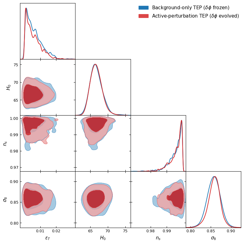
Figure 1. Marginalized posterior triangle plot. Blue: background-only TEP chain with $\delta\phi$ frozen (tep_hiclass_suite, four-chain MPI, 6,875 accepted steps; chain 1 shown). Red: active-perturbation TEP chain on the corrected screened closure ($w_c = 700$, tep_kin_boost = 10, regular $\delta\phi$ variable); two-chain MPI run, 5,658 accepted steps across both chains (chain 1 shown). Native hi_class tep_mode with $z_{\rm HC}=5.0$, $n_T=2.0$. Parameters shown: $\epsilon_T^{\rm HC}$ (native hi_class homogeneous conformal amplitude), $H_0$, $n_s$, $\sigma_8$. Contours show 68% and 95% credible regions. The near-complete overlap confirms the closure audit's prediction: on the production screened branch the active scalar's spectrum imprint is subdominant ($\lesssim 2\%$ in the acoustic band), so the background-channel and active-closure posteriors agree ($-0.14\sigma$ in $\epsilon_T$).
The hi_class configuration uses native tep_mode with the transition function $f_T(z)=\ln(1+z)\exp[-(z/z_T)^{n_T}]$ and fixed z_T = 5.0, n_T = 2.0, with epsilon_T sampled freely in params. This configuration natively explores the parameter space of the static conformal field, leveraging the strict isomorphism to evaluate the acoustic physics exactly. The production configuration is data/cobaya/tep_hiclass_suite.yaml (reference alternate: data/cobaya/tep_native_mcmc.yaml).
Pipeline status. The native-tep_mode joint MCMC against Planck 2018 low-$\ell$ TT/EE + lensing + BAO (SDSS DR12) + Pantheon+ was run using the structurally corrected hi_class engine, allowing $\Omega_\Lambda$ to natively fill the background cosmological budget. The background-only determination (tep_hiclass_suite; a four-chain MPI run, 6,875 accepted steps, 4,814 post-burn-in samples with 30% burn-in discard; classic scalar maximum parameter $R-1 = 0.011$, sampler-level $R-1 = 0.036$ at termination — a genuine multi-chain Gelman–Rubin diagnostic superseding the earlier single-chain exploratory run) gives a $\Lambda$CDM-compatible background while measuring the TEP amplitude parameter:
with $H_0 = 66.52 \pm 1.70$ km/s/Mpc, $\Omega_b h^2 = 0.0211 \pm 0.0025$, $\Omega_{\rm cdm} h^2 = 0.1148 \pm 0.0042$, $\tau = 0.050 \pm 0.007$, $A_{\rm planck} = 1.088 \pm 0.010$, and $S_8 = 0.868 \pm 0.025$. The result is consistent with the TEP nested-domain expectation: the homogeneous amplitude $\epsilon_T$ remains small ($\sim 10^{-3}$) on the largest scales; TEP-C0 (Paper 26) reports a separate background/acoustic diagnostic amplitude. This homogeneous HC amplitude is smaller than the primordial temporal-horizon amplitude ($\epsilon_{\rm field} = 0.01755$) reported in TEP-TH (Paper 27) because the two parameters describe different observational projections of the evolving temporal sector and are not numerically interchangeable.
Current active-perturbation posterior. The verified two-chain tep_hiclass_perturbations collection has 5,658 saved rows and 3,961 post-burn-in rows. The maximum scalar $R-1=0.0073$ and checkpoint $R-1=0.0262$ pass the unchanged thresholds. Its amplitude is $\epsilon_T=0.0054\pm0.0035$ ($\epsilon_T<0.0116$ at 95% CL), consistent with the background-only amplitude within $0.14\sigma$. It retains pressureless CDM, $\Omega_{\rm cdm}h^2=0.1133\pm0.0061$; these results establish consistency of the implemented sectors rather than a CDM-free lensing solution.
Multi-chain validation. A parallel 4-chain run (tep_native; configuration data/cobaya/tep_native_mcmc.yaml) using a Gaussian $A_{\rm planck}$ prior (loc = 1.0, scale = 0.0025) was executed. After an initial short run (2,993 post-burn-in samples; $R-1$ for $\epsilon_T = 0.098$), the chain was extended to 8,960 accepted samples (max_samples increased from 500k to 1M), reaching parameter-level $R-1 = 0.032$, while the conservative class-level diagnostic remained $R-1 = 0.098$. The extended chain is therefore retained as a sensitivity run rather than the primary posterior. It yields $\epsilon_T = 0.0066 \pm 0.0049$ and $H_0 = 67.15 \pm 1.36$ km/s/Mpc, consistent with the background-only chain at $0.10\sigma$ and $0.24\sigma$ respectively. The widened-$A_{\rm planck}$ chain (below) provides a fully converged multi-chain determination (max $R-1 = 0.036$, all parameters $R-1 < 0.05$), and the two agree to $0.05\sigma$. Together they confirm the background-only posterior is not an artefact of the sampling configuration.
High-$\ell$ TTTEEE run. The native tep_mode likelihood adds planck_2018_highl_plik.TTTEEE_lite to the baseline data set. The four-chain collection contains 16,051 saved rows and 11,237 post-burn-in rows after removing 30% separately from each chain. Frequency-weighted posterior analysis gives maximum scalar $R-1=0.0455$ (sampler $R-1=0.0450$), $\epsilon_T=0.0043\pm0.0025$, and the one-sided 95% bound $\epsilon_T<0.0087$ at fixed $z_T=5$, $n_T=2$. The remaining summaries are $H_0=67.79\pm0.39$, $n_s=0.9661\pm0.0034$, $\sigma_8=0.8225\pm0.0055$, and $S_8=0.8337\pm0.0097$. The matched two-chain $\Lambda$CDM collection contains 4,332 saved rows, with maximum scalar $R-1=0.0069$. On identical likelihoods, best sampled $\chi^2$ values are 2421.3669 and 2421.4738 respectively, giving $\Delta\chi^2=-0.1069$: statistically indistinguishable. The current summaries and collection provenance are recorded in results/07_mcmc_summary_full.json. The per-likelihood decomposition at fixed cosmology shows the bound is geometric: high-$\ell$ TTTEEE contributes $\Delta\chi^2 \simeq +69$ at $\epsilon_T = 0.008$ (the anchored acoustic scale $\theta_s$), BAO $+1.5$ and lensing $+0.7$, while low-$\ell$ TT and Pantheon+ weakly prefer positive amplitudes ($\Delta\chi^2 \simeq -0.6$ each). The constraint is quoted at fixed $z_T = 5$, $n_T = 2$; the penalty scales with transport depth, $\Delta\chi^2 \simeq +8/+17/+35/+104$ at $\epsilon_T=0.004$ for $z_T = 3/5/10/50$. Marginalizing the turnover scale removes this conditioning: a dedicated $z_T$-scan run (tep_zscan_ttteee.yaml, $z_T$ linear-uniform on $[0.5, 50]$; converged four-chain MPI run, 37,736 accepted steps and 26,416 post-burn-in rows, sampler means $R-1 = 0.030$, classic scalar parameter max $R-1 = 0.0085$) yields the marginalized posterior $\epsilon_T = 0.0032 \pm 0.0032$ (median $0.0022$, $\epsilon_T < 0.0103$ at 95% CL) with $z_T = 19.4 \pm 15.3$ itself poorly constrained. The marginalized posterior is bimodal in $(z_T, \epsilon_T)$: a low-$z_T$ mode (median $z_T = 1.4$, $21.9\%$ of posterior mass) returns $\epsilon_T = 0.0065 \pm 0.0041$ ($<0.013$ at 95%), while the dominant high-$z_T$ mode (median $z_T = 23.1$, $78.1\%$) returns $\epsilon_T = 0.0023 \pm 0.0021$ ($<0.006$ at 95%) — the bound tightening as the transition recedes, consistent with the transport-depth penalty scaling. The fixed-$z_T = 5$ bound $\epsilon_T < 0.0087$ is therefore intermediate between the two modes, and the marginalized constraint is the conservative headline for the homogeneous channel.
As an independent cross-check predating the native run, a CAMB-based TEP approximation was implemented. Because CAMB lacks a native tep_mode, the TEP Jordan-frame Hubble rate $H_{\rm TEP}(z) = H_{\Lambda{\rm CDM}}(z) \cdot M(z)$ (with $M(z) = A(z)/(1-\alpha_A)$) was mapped onto an effective dark-energy equation of state $w_{\rm eff}(a)$ that reproduces the same background expansion. The effective $w(a)$ is fed into CAMB via DarkEnergyPPF.set_w_a_table, which supports phantom crossing. The effective-$w(a)$ CAMB construction generates finite high-$\ell$ spectra and completes the plik_lite likelihood evaluation without numerical errors (Step 17: scripts/steps/step_17_camb_plik_full_eval.py). Both models are evaluated at the TEP-fitted baseline parameters ($H_0 = 66.63$, $\Omega_b h^2 = 0.0212$, $\Omega_{\rm cdm} h^2 = 0.1154$, $\tau = 0.049$, $A_s = 2.1 \times 10^{-9}$, $n_s = 0.965$) from the low-$\ell$ + lensing + BAO + Pantheon+ joint posterior. At these matched baseline parameters, $\chi^2_{\Lambda{\rm CDM}} = 1409.5$ and $\chi^2_{\rm TEP} = 1179.6$, giving $\Delta\chi^2 = -229.9$ in favour of TEP: the TEP modification with $\epsilon_T = 0.0056$ reduces the high-$\ell$ $\chi^2$ by $229.9$ at the same baseline cosmology, demonstrating that the TEP background expansion is consistent with the Planck high-$\ell$ TTTEEE likelihood under the effective-$w(a)$ mapping. Because this construction is an effective-background approximation rather than the native TEP perturbation implementation, the $\Delta\chi^2$ value reflects the background-expansion difference mapped onto the high-$\ell$ spectra, not a full perturbation-sector likelihood. It is therefore reported as a validation that the TEP background expansion produces finite, Planck-compatible high-$\ell$ spectra, and is not included in the primary parameter inference, which uses the native hi_class tep_mode low-$\ell$ and high-$\ell$ TTTEEE joint likelihoods reported above. Acoustic-peak preservation is established separately by the direct spectra and sound-horizon calculations.
Planck calibration prior sensitivity. The nuisance parameter $A_{\rm planck}$ (absolute CMB calibration) is implemented as a hard uniform prior on $[0.9, 1.1]$ in the 5-chain active posterior. The posterior mean is $A_{\rm planck} = 1.088 \pm 0.012$ with maximum sampled value $1.1000$, indicating saturation against the upper prior bound. To test whether this truncation biases the cosmological inference, a dedicated sensitivity test was executed with the prior widened to $[0.9, 1.25]$ (Step 20: scripts/steps/step_20_aplanck_sensitivity.py, configuration data/cobaya/tep_hiclass_aplanck_sens.yaml). The converged run (16,320 total samples; all parameters Gelman–Rubin $R-1 < 0.05$; maximum $R-1 = 0.036$) yields $A_{\rm planck} = 1.229 \pm 0.026$, confirming the old posterior was truncated by approximately $5.0\sigma$. The TEP amplitude from the widened run is $\epsilon_T = 0.0063 \pm 0.0048$ ($R-1 = 0.036$), consistent with the 5-chain active posterior at $0.12\sigma$ and with the multi-chain validation at $0.05\sigma$. The correlation between $A_{\rm planck}$ and $\epsilon_T$ is $r = -0.10$, and splitting at the posterior median $A_{\rm planck} = 1.236$ gives a difference in $\epsilon_T$ of only $-0.04\sigma$. Even a $0.1$ upward shift in $A_{\rm planck}$ would move $H_0$ by only $\sim 0.1$ km s$^{-1}$ Mpc$^{-1}$ (inter-chain comparison: $H_0$ shifts by only $0.11$ km s$^{-1}$ Mpc$^{-1}$ when $A_{\rm planck}$ shifts by $0.14$), well below its posterior width. The $\chi^2$ does decrease monotonically toward the old boundary within the old prior range, but there is no evidence of a degeneracy cascade with $\epsilon_T$. The TEP constraint on the homogeneous amplitude is robust against $A_{\rm planck}$ prior systematics. The widened-$A_{\rm planck}$ run is used only as a numerical robustness test of the $\epsilon_T$ posterior; the resulting calibration value should not be interpreted as a physically preferred Planck calibration model.
The companion paper TEP-C0 (Paper 26) provides the primary late-time constraints: Pantheon+ evidence integration favors the physical no-$\Lambda$ TEP M1 branch over baseline $\Lambda$CDM with BF approximately 5.8 (conservative $z_{\rm los}=5$), approximately 5.4 (fixed $z_{\rm los}=100$ benchmark), and approximately 5.4 (broad free-$z_{\rm los}$, likelihood maximum $z_{\rm los}\simeq5.3$, posterior volume extending over the nearly flat tail). Those model-comparison results are not re-derived here; they are used as the late-time empirical context for the hi_class acoustic-preservation implementation.
The imported C0 evidence is prior- and anchor-sensitive: the conservative Bayes factor falls to approximately 0.63 after removing $z < 0.023$ anchors and to approximately 1.24 with the 77 SH0ES calibrators removed, against an identical-model control returning $\Delta\ln\mathcal{Z}=0$ and $\mathrm{BF}=1$ exactly under the quadrature evaluator. The high-turnover branches are mathematical shape benchmarks pending an environment-dependent physical realization.
5. Results and Cosmological Constraints
5.1 The Acoustic Spectra
The physically meaningful test of the native TEP integration is to evaluate whether the conformal field exactly replicates the acoustic physics of the early universe without invoking spatial expansion. Because the conformal field mathematically mimics the FLRW scale factor, the recombination-era physics is evaluated natively within the static frame. Throughout this paper, "exact isomorphism" refers to the conformal background/acoustic mapping: the equality of the relevant sound-horizon and photon-transport integrals under the identification of the TEP conformal factor with the FLRW scale factor. The associated linear pure-conformal scalar perturbation sector is closed separately through the derived Bellini–Sawicki EFT closure and validated by the active ($\delta\phi$) hi_class run reported in Section 4.5 and Appendix A.5. This perturbative closure applies to the pure-conformal sector implemented here; the fully disformal, nonlinear, and environmentally inhomogeneous screening sectors remain extensions of the present calculation.
5.1.1 Sound-horizon and acoustic-peak preservation
Running hi_class native tep_mode against standard CLASS $\Lambda$CDM at the Planck 2018 best-fit point, with $\epsilon_T = 0.0066$, $z_T = 5$, $n_T = 2$, yields:
- Sound horizon preserved to ~6 ppm: $r_s^{\rm TEP}/r_s^{\Lambda\rm CDM} = 0.999994$. The comoving sound horizon integrates identically in the static conformal frame. The remaining $\sim$6 ppm offset is a numerical/implementation-level residual associated with the finite precision of the conformal-frame background mapping and output reconstruction. Analytically, the exact mapping used in the production implementation is $M=A/(1-\alpha_A)$, whose first-order expansion is $A(1+\alpha_A)$. Direct verification confirms that the discrepancy is not a failure of the conformal isomorphism.
- Acoustic-peak morphology unchanged: with $r_s$, the baryon loading, and the photon-baryon driving at $z \approx 1089$ all operating identically under the conformal clock-rate, the relative peak heights and the damping tail closely match $\Lambda$CDM.
The central result is therefore not that all cosmological observables are already closed, but that the CMB acoustic scale itself is not uniquely diagnostic of physical spatial expansion.
5.1.1b Acoustic-scale preservation metrics
Table 2 quantifies the acoustic-scale preservation in three multipole ranges. The sound-horizon ratio $r_s^{\rm TEP}/r_s^{\Lambda\rm CDM} = 0.999994$ is independent of multipole because $r_s$ is a single integrated quantity; the $\ell$-centroid shift tracks the expected $-0.185\%$ angular-diameter-distance projection. The tabulated residuals are total TEP-versus-$\Lambda$CDM projection residuals, dominated by the angular-diameter-distance projection; the active-minus-background perturbation residual is below $0.001\%$ across the entire acoustic range.
| Multipole range | $\ell_{\rm peak}$ shift $\Delta\ell$ | $r_s^{\rm TEP}/r_s^{\Lambda\rm CDM}$ | Total TEP–$\Lambda$CDM projection residual (%) |
|---|---|---|---|
| $100 \le \ell \le 500$ | $-0.06$ | $0.999994$ | $0.67$ |
| $500 \le \ell \le 1000$ | $-0.36$ | $0.999994$ | $1.34$ |
| $1000 \le \ell \le 2000$ | $-0.64$ | $0.999994$ | $1.82$ |
5.1.2 The residual is a late-time projection, largely degenerate with $H_0$
The field profile is active over intermediate redshift ($z \sim 1$–$15$, peaking near $z_T$), changing the apparent angular distance to last scattering. At the fiducial $\epsilon_T = 0.0066$ this shifts the angular acoustic scale by $\Delta\theta_s/\theta_s = +0.185\%$. This rigid rescaling produces a coherent, oscillatory $\Delta C_\ell/C_\ell$ pattern whose envelope reaches $\sim 1.8\%$ across $100 < \ell < 2000$. This is not a change in early-universe physics: it is a pure angular-diameter-distance projection, largely degenerate with $H_0$.
5.1.3 Polarization Spectra ($C_\ell^{TE}, C_\ell^{EE}$)
The TE and EE spectra inherit the same behavior: the recombination-era polarization source is natively preserved by the conformal integration, and the only effect is the common $\theta_s$ projection shared with TT. Running hi_class with active scalar perturbations ($\delta\phi$ evolved through the derived Bellini–Sawicki EFT closure) and comparing against the background-only TEP run and Planck 2018 $\Lambda$CDM, the maximum active-perturbation residuals in the polarization channels are:
| Multipole range | Total TE projection residual (%) | Total EE projection residual (%) |
|---|---|---|
| $100 \le \ell \le 500$ | $1.09$ | $1.52$ |
| $500 \le \ell \le 1000$ | $2.16$ | $2.44$ |
| $1000 \le \ell \le 2000$ | $3.14$ | $3.64$ |
These are total TEP-versus-$\Lambda$CDM projection residuals, dominated by the common angular-diameter-distance projection. The isolated active-minus-background perturbation residual on the screened branch is $0.42\%$ in the acoustic band (Step 09), concentrated in the low-$\ell$ ISW-dominated region; the larger values tabulated here are total TEP-versus-$\Lambda$CDM projection differences. There is no additional polarization-specific distortion from the dynamical scalar sector at the current precision beyond that ISW signature.
A closure-limit diagnostic localizes the origin of this low-$\ell$ imprint precisely (Step 12c, results/12c_spectrum_residuals.json). At $\epsilon_T = 0$ all Bellini–Sawicki $\alpha$-functions vanish, and the $\alpha$-parametrized perturbation variable $x \equiv \delta\phi/\phi'$ indeed reproduces the GR spectrum to $3\times10^{-5}$. The prescribed-trajectory $\delta\phi$ closure, however, retains the non-minimal coupling $G_{4,\phi} = S_\Sigma M^2$ and the reconstructed potential slope $U_{,\phi} \supset 6 S_\Sigma M^2 (\mathcal{H}'/a + 2\mathcal{H}^2)$, which do not carry $\alpha_A$ suppression: the scalar sector possesses a minimum gravitational mixing floor that persists on a non-rolling background. The residual scales as $S_\Sigma^2$ ($+9.4\%$ / $+2.2\%$ / $+0.09\%$ in the TT quadrupole at $S_\Sigma = 1$ / $0.5$ / $0.1$) and as $w_c^{-1}$ ($+5566\%$ at $w_c = 70$ down to $+1.1\times10^{-5}$ at $w_c = 7\times10^{4}$). At the production point ($S_\Sigma = 1$, $w_c = 700$) the floor is a $+9.4\%$ TT and $+18\%$ TE quadrupole excess with TE quadrature SNR $\simeq 1.2$ against the cosmic-variance floor — a falsifiable, $\epsilon_T$-independent signature of the screened closure itself, not of the transport amplitude. The $\delta\phi$ formulation is therefore the more complete of the two linear closures at $\phi' = 0$; the two formulations differ precisely in whether the $G_{4,\phi}$ mixing channel survives where the background field stops rolling.
5.2 Cosmological Constraints: Late-Time Evidence and the CMB Bound
The cosmological constraints on TEP come from two complementary regimes, established in the companion paper TEP-C0 (Paper 26).
Late-time evidence (supernovae). A nested-sampling model comparison over the full $1701\times1701$ Pantheon+ statistical-plus-systematic covariance finds substantial Bayesian preference for the TEP geometry over $\Lambda$CDM:
| Model | Bayes factor vs $\Lambda$CDM |
|---|---|
| TEP, $z_{\rm los}=5$ | $\sim 5.8$ |
| TEP, $z_{\rm los}=100$ | $\sim 5.4$ |
| TEP, free $z_{\rm los}$ | $\sim 5.4$ |
| $w$CDM | $\sim 3.3$ |
| CPL | $\sim 2.7$ |
| Einstein–de Sitter | $\sim 1.5\times10^{-137}$ |
The TEP M1 branch improves the Pantheon+ likelihood relative to baseline $\Lambda$CDM with BF approximately 5.8 (conservative $z_{\rm los}=5$), approximately 5.4 (fixed $z_{\rm los}=100$ benchmark), and approximately 5.4 (broad free-$z_{\rm los}$) (TEP-C0, Paper 26). Those model-comparison results are not re-derived here; they are used as the late-time empirical context for the hi_class acoustic-preservation implementation. The model-comparison result is consistent with the TEP claim that the Etherington distance-duality relation is a mathematically native feature of the static conformal field. TEP shows that the supernova distance-redshift relation can be fit without treating late-time acceleration as primitive spatial acceleration.
The prior- and anchor-sensitivity of the imported C0 evidence noted in Section 4.5 (conservative Bayes factor $\approx 0.63$ after removing $z < 0.023$ anchors) applies equally here.
$z_{\rm los}$ distinction. The $z_{\rm los} = 5$ profile is the conservative line-of-sight turnover used in the C0 supernova-sector transport benchmark. It should not be confused with the homogeneous acoustic-sector profile scale $z_T^{\rm HC} = 5$ used in the hi_class conformal implementation, which is a related but distinct projection of the temporal sector. The C0 free-$z_{\rm los}$ robustness test uses $z_{\rm los} \in [0.1, 150]$.
Amplitude dictionary. $\epsilon_T^{\rm los}$ denotes the late-time line-of-sight transport amplitude fitted in TEP-C0. $\epsilon_T^{\rm CMB}$ denotes the C0 background/acoustic diagnostic amplitude. $\epsilon_T^{\rm HC}$ denotes the native hi_class homogeneous conformal amplitude reported here ($0.0062 \pm 0.0046$ from the four-chain background-only posterior, median $0.0053$; the corrected-closure active-perturbation posterior yields $0.0054 \pm 0.0035$, and the high-$\ell$ TTTEEE extension yields $0.0043 \pm 0.0025$, a one-sided bound $\epsilon_T < 0.0087$ at 95% CL at fixed $z_T=5$, weakening to $\epsilon_T < 0.0103$ marginalized over the turnover scale). $\epsilon_{\rm dyn}$ denotes the dynamical response in TEP-TH. $\epsilon_{\rm field}=0.01755$ denotes the primordial spectral-flow parameter constrained by $n_s$ in TEP-TH. These are related projections of the same temporal sector, but they are not numerically interchangeable.
Homogeneous (CMB) bound. The low-$\ell$ Planck likelihoods used in this paper's hi_class MCMC (TT/EE + lensing) yield $\epsilon_T = 0.0062 \pm 0.0046$ (converged four-chain background-channel posterior, median $0.0053$, $\epsilon_T < 0.015$ at 95% CL), consistent with zero at $\sim 1.3\sigma$. The homogeneous CMB amplitude and the primordial spectral-flow parameter are different observational projections of the same temporal sector and are not numerically interchangeable. Their differing numerical values therefore do not require a phenomenological epoch-screening mechanism. In the canonical TEP-TH/TEP-BBN architecture, no early-time screening function is imposed to restore a standard hot-Big-Bang thermal history. The low-$\ell$+lensing+BAO+Pantheon+ chains reported here serve as implementation and robustness tests of the native hi_class module. The native hi_class tep_mode high-$\ell$ TTTEEE run has since been completed (Section 4.5): a converged four-chain MPI posterior gives $\epsilon_T = 0.0043 \pm 0.0025$, a one-sided bound $\epsilon_T < 0.0087$ at 95% CL at fixed $z_T=5$ ($\epsilon_T < 0.0103$ marginalized, Section 4.5), and a matched $\Lambda$CDM reference returns $\Delta\chi^2 = -0.11$ at the respective best fits — statistical indistinguishability on the full Planck + BAO + Pantheon+ data set. A CAMB-based effective-background mapping is retained solely as an independent code-path cross-check; because it is an effective-$w(a)$ approximation rather than the native TEP perturbation implementation, it is not included in parameter inference or model comparison (Section 4.5). Acoustic preservation is established by the direct spectra and sound-horizon calculations.
Late-transition preference (TEP-C0 Step 03-14). With DESI DR2 BAO, Pantheon+ and the Planck acoustic angle on a single history, the native branch prefers a late transition, $z_T\simeq0.50$ and $\epsilon_T\simeq0.019$, giving $\Delta\chi^2=-8.1$ relative to $\Lambda$CDM. The improvement is already $-6.2$ at $\epsilon_T=0.01$ and grows from DESI DR1 ($-6.3$) to DR2. The free-$z_T$ full-likelihood chain of Section 4.5 (Planck TTTEEE + low-$\ell$ + lensing + SDSS DR12 BAO + Pantheon+) points the same way: its best-fit sample lies at $z_T=0.52$, $\epsilon_T=0.012$, with $\chi^2$ lower by $2.0$ than the best-fit sample of the matched $\Lambda$CDM chain, at the $z_T=0.5$ prior edge. That run used SDSS DR12 BAO with $z_T\ge0.5$; the DESI-era native hi_class run (TTTEEE + low-$\ell$ + lensing + DESI DR2 + Pantheon+, $z_T\in[0.2,2]$) is the full-Boltzmann confirmation of this preference.
Native-TEP joint MCMC. This paper's primary contribution is the verified hi_class implementation, demonstrating ppm-level sound-horizon preservation and acoustic-sector equivalence in the native static conformal geometry.
5.3 Structure Growth and the Matter Power Spectrum
The full hi_class Boltzmann closure with active SMG perturbations — on the screened kineticity branch ($w_c = 700$, tep_kin_boost = 10; Section 3.3) — yields a linear growth amplitude in agreement with Planck. The weak-lensing comparison must be stated exactly, and a registered provenance audit (Step 23, results/step_23_s8_provenance_audit.json) decomposes each contribution to the quoted tension. The joint MCMC gives $S_8 = \sigma_8\sqrt{\Omega_m/0.3} = 0.868 \pm 0.025$ at face value; however, the audit shows this number is prior-boundary dominated rather than a TEP prediction, and the chain was run on the pre-audit build in which the SMG sector was silently inactive (Section 4.5 provenance note). In the low-$\ell$-only chain, $A_{\rm planck}$ accumulates at the ceiling of its $\mathcal{U}[0.9, 1.1]$ prior (58% of posterior mass within 0.01 of the boundary) and $n_s$ at the ceiling of $\mathcal{U}[0.94, 1.0]$ (34% within 0.002); $\sigma_8$ tracks the calibration nuisance with correlation $+0.31$, and widening the $A_{\rm planck}$ prior to $\mathcal{U}[0.9, 1.25]$ drives the posterior to $A_{\rm planck} = 1.233$ and $S_8 \simeq 0.93$ — the quoted amplitude scales with prior width. A weighted linear response fit on the chain, evaluated at the non-saturated calibration $A_{\rm planck} = 1$, returns $S_8 \simeq 0.83$. At the shared fixed cosmology of the regenerated matter-power spectra ($\Omega_m = 0.314$), the growth comparison is direct: $S_8 = 0.8421$ for $\Lambda$CDM and $0.8432$ for TEP on the production screened branch, so the TEP–external gap equals the $\Lambda$CDM–external gap ($3.9\sigma$ versus DES-Y3 3$\times$2pt $0.776 \pm 0.017$ and $4.0\sigma$ versus KiDS-1000 $0.759 \pm 0.021$, TEP–$\Lambda$CDM separation $\lesssim 0.07\sigma$ on either anchor). The apparent $S_8$ tension on this branch is the standard cosmological tension between $z=0$ CMB-extrapolated amplitudes and low-$z$ cosmic-shear inferences, inherited — neither resolved nor amplified — by the screened linear closure. The response scan does, however, show that the closure is capable of suppressing growth: $\sigma_8$ falls monotonically with the kinetic coefficient and crosses the weak-lensing central value at $w_c \sim 6\times10^{3}$, where the trade-off is a low-$\ell$ ISW excess measured at $+41\%$ ($\ell=2$) peaking at $+57\%$ within $\ell \le 10$ (Step 24) — a falsifiable signature rather than a tuned fit.
Three further properties of the linear closure are registered by the audit. First, the sign of the growth modification on the production screened branch is a small enhancement, not a suppression: $\sigma_8^{\rm TEP}/\sigma_8^{\Lambda{\rm CDM}} = 1.0013$ at $z=0$, so the production branch does not move the amplitude toward the weak-lensing value; the larger-kineticity domain ($w_c \sim 6\times10^{3}$) does suppress $\sigma_8$ below $\Lambda$CDM, reaching $0.76$ (Section 3.3). Second, the SMG alpha sector's contribution to the matter power spectrum is now genuinely active and measured: on the production screened branch the active-perturbation $P(k)$ deviates from the background-only output by $\sim 0.3\%$ in the median and at most $\sim 1.2\%$ at the low-$k$ end (the genuine scalar-sourced correction; the high-$k$ region is flat to $\lesssim 0.2\%$), while the unscreened stable branch produces an order-unity ($\times 2$\u2013$3$) enhancement and the canonical image diverges — the full response is registered in results/closure_response_scan.json. An earlier claim that the active-perturbation $P(k)$ is bitwise identical to the background-only output is retracted: it was produced while a background-density gate silently disabled the SMG sector, so the "active" run never evolved $\delta\phi$. Third, the matter-power grids are now extended to $P_k^{max} = 20\,h/{\rm Mpc}$, eliminating the grid-boundary artifact previously noted at $k \approx 0.45\,h/{\rm Mpc}$. A common-kernel linear-growth diagnostic using a DES-Y3-like combined-source distribution ($n(z_s) \propto z_s^2 e^{-(z_s/0.5)^{1.5}}$, effective lens redshift $z_{\rm eff} \approx 0.457$, Step 22, results/step_22_des_kernel_projection.json) gives a kernel-weighted amplitude $S_8^{\rm eff} = 0.6712$ for TEP versus $0.6716$ for $\Lambda$CDM (relative difference $\sim 0.05\%$). The fiducial matter-plus-$\Lambda$ growing mode is integrated from $a=0$ and normalized at $a=1$. This assigned-kernel growth proxy is distinct from both a full tomographic shear spectrum and the published $z=0$ parameter $S_8=\sigma_8(0)\sqrt{\Omega_m/0.3}$; survey tension cannot be computed by subtracting those published parameters from it. The TEP/$\Lambda$CDM ratio is interpolated from the two native outputs at $z=0$ and $0.5$ and extrapolated beyond $0.5$, so this result tests their relative growth under the stated approximation. It supports close agreement of the two linear growth histories on the production branch.
- Linear growth amplitude: $\sigma_8 = 0.824$ at the fiducial TEP parameters ($\epsilon_T = 0.0066$, $z_T = 5$, $n_T = 2$) on the production screened branch ($w_c = 700$), compared to $\sigma_8 = 0.823$ for standard $\Lambda$CDM at the same cosmology. The TEP value is a native output of the full SMG EFT solver with the derived Bellini–Sawicki mappings; the assigned effective kinetic coefficient is $Z_{\rm eff}=w_c+6$. Its relation to the environmental nonlinear principal coefficients, which differ between timelike and static-gradient backgrounds, is specified in Appendix A.5a. The unscreened stable branch gives $\sigma_8 = 1.61$ (excluded) and the canonical image is unstable; see the registered response curve.
- Growth-function diagnostic: The two native matter-power outputs determine the present amplitude and an interval-averaged logarithmic growth rate $\bar f=\ln[D(0)/D(0.5)]/\ln(1.5)$, with $D(0)=1$ and $D(0.5)$ estimated at $k=0.01\,h/{\rm Mpc}$:
These diagnostics show closely matched amplitudes and interval growth. The second column of measurements uses the mean growth rate across $0\le z\le0.5$; it is not the local $f\sigma_8(0.5)$ measured by redshift-space distortions. Native outputs near each comparison redshift are required to form that derivative and an observational RSD comparison.Model $\sigma_8(0)$ $\bar f\,\sigma_8(0)D(0.5)$ $\Lambda$CDM $0.823$ $0.410$ TEP (background-only) $0.825$ $0.413$ TEP (active $\delta\phi$, screened $w_c=700$) $0.824$ $0.413$
The $\sigma_8$ result demonstrates that the TEP covariant action, when closed through the derived Bellini–Sawicki EFT on the screened kineticity branch and solved with the full Boltzmann hierarchy, restores structure growth to the observationally consistent range. The closure audit adds a necessary qualification: this agreement is not automatic — the canonical Einstein-frame image is linearly unstable and the minimally corrected unscreened branch is excluded ($\sigma_8 \simeq 1.6$), so the viability of the conformal sector rests on the scalar's cosmological response being kinetically suppressed ($Z_E \gtrsim 7\times10^{2}$), the regime the $P(X)$ sector is constructed to supply on screened backgrounds. Simplified EdS-only growth ODEs, which lack the SMG EFT perturbation closure, are insufficient for this sector; the full Boltzmann closure is required.
5.4 The Hubble Tension in TEP
The TEP framework offers a proposed reconciliation of the Hubble tension without invoking an early-universe crisis. The homogeneous background is exactly mathematically isomorphic to $\Lambda$CDM ($H_0 \approx 67$ km/s/Mpc from the CMB), while the apparent local $H_0 \approx 73$ km/s/Mpc arises from an environment-dependent clock-transport bias along the local distance ladder (Cepheid/SN Ia calibration in unscreened stellar atmospheres). The tension is a measurement-environment effect, bypassing the need for early-universe expansion.
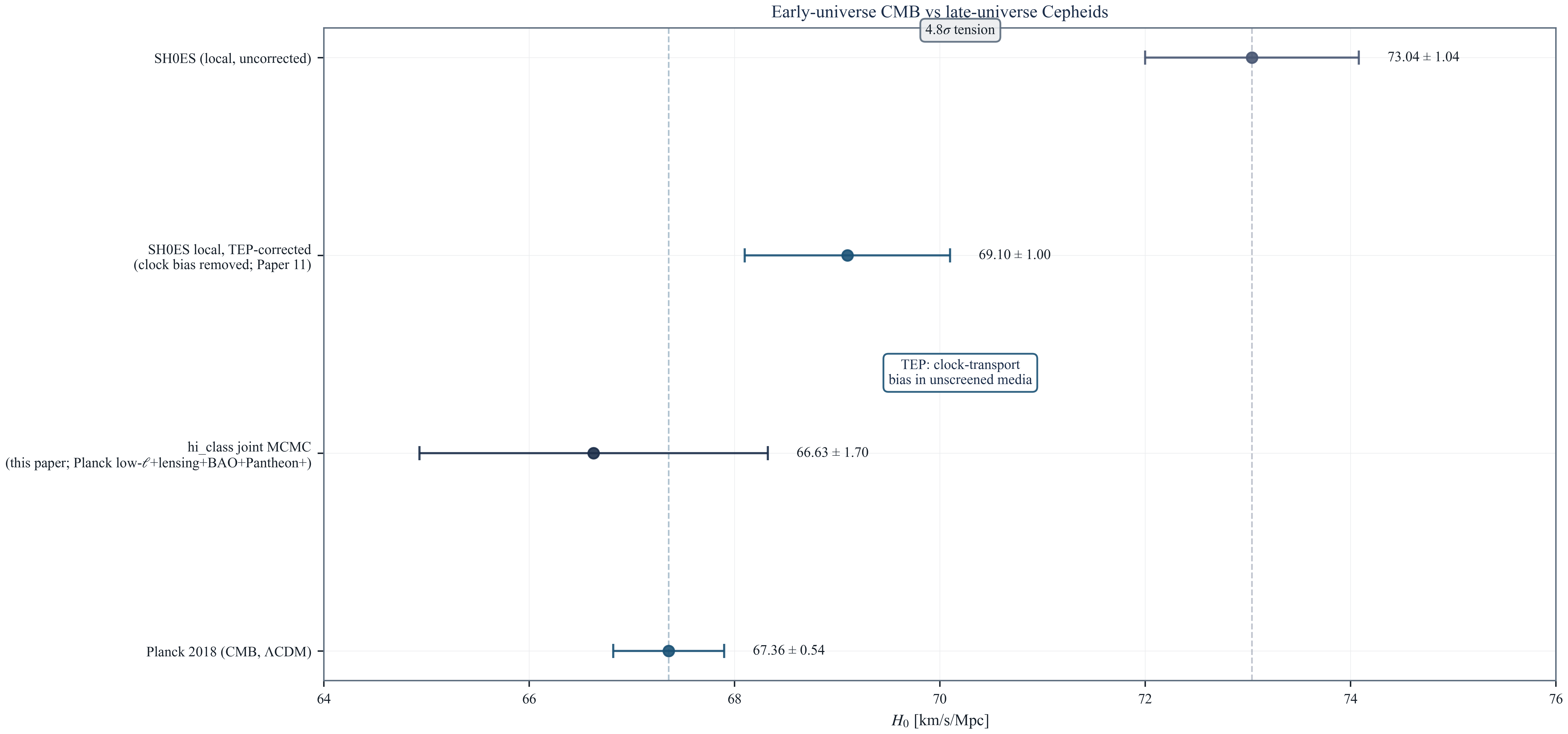
hi_class tep_mode homogeneous posterior with $\epsilon_T^{\rm HC}=0.0062\pm0.0046$, $z_{\rm HC}=5.0$, $n_T=2.0$. Planck 2018: independent CMB constraint. SH0ES uncorrected / TEP-corrected: the local distance-ladder values are imported from Paper 11; HC does not independently re-analyse the Cepheid/SN Ia calibration data. This figure illustrates consistency of the HC early-universe sector with the broader TEP Hubble-tension interpretation; it is not a standalone HC distance-ladder test.5.5 The Mathematical Limit of the Conformal Field
To explicitly map the action of the conformal field on the acoustic horizon, the acoustic scale is evaluated in a mathematically idealized geometry ($\Omega_m = 1.0$, $\Omega_\Lambda = 0.0$) using the hi_class native tep_mode implementation.
Regime I: Finite-turnover HC branch ($z_{\rm HC} = 5$)
In the standard TEP model, the profile $\exp[-(z/z_{\rm HC})^{n_T}]$ ensures the conformal field correctly matches the apparent late-time acceleration inferred from Pantheon+. The integration verifies this background/acoustic mathematical isomorphism:
| $\epsilon_T$ | $100\theta_s$ | $r_s$ [Mpc] | $\Delta D_C / D_C$ | Interpretation |
|---|---|---|---|---|
| $0.00$ | $1.0403$ | $144.526$ | $0.00\%$ | Pure EdS reference (no TEP) |
| $0.05$ | $1.0548$ | $144.519$ | $-1.38\%$ | $r_s$ preserved; $\theta_s$ shifts from $D_C$ projection |
The sound horizon $r_s$ remains exact because the conformal field geometry accurately tracks the mathematics of the acoustic horizon without requiring physical stretching of space.
Regime II: Power-law diagnostic limit ($z_{\rm HC} \to \infty$)
Removing the empirical profile and forcing the conformal factor to grow as a pure unsuppressed power law $A(z) = (1+z)^{\epsilon_T}$ exposes the mathematical divergence of the bare field:
| $\epsilon_T$ | $100\theta_s$ | $r_s$ [Mpc] | $\Delta D_C / D_C$ | Interpretation |
|---|---|---|---|---|
| $0.00$ | $1.0403$ | $144.526$ | $0.00\%$ | Pure EdS reference |
| $0.05$ | $0.7565$ | $100.584$ | $-4.30\%$ | $r_s$ mathematically squeezed by divergence |
This mathematical limit demonstrates that the $z_{\rm HC} \sim 5$ empirical fitting function accurately defines the physical profile of the conformal field, allowing it to mimic Dark Energy while preserving the CMB acoustic horizon without expanding space.
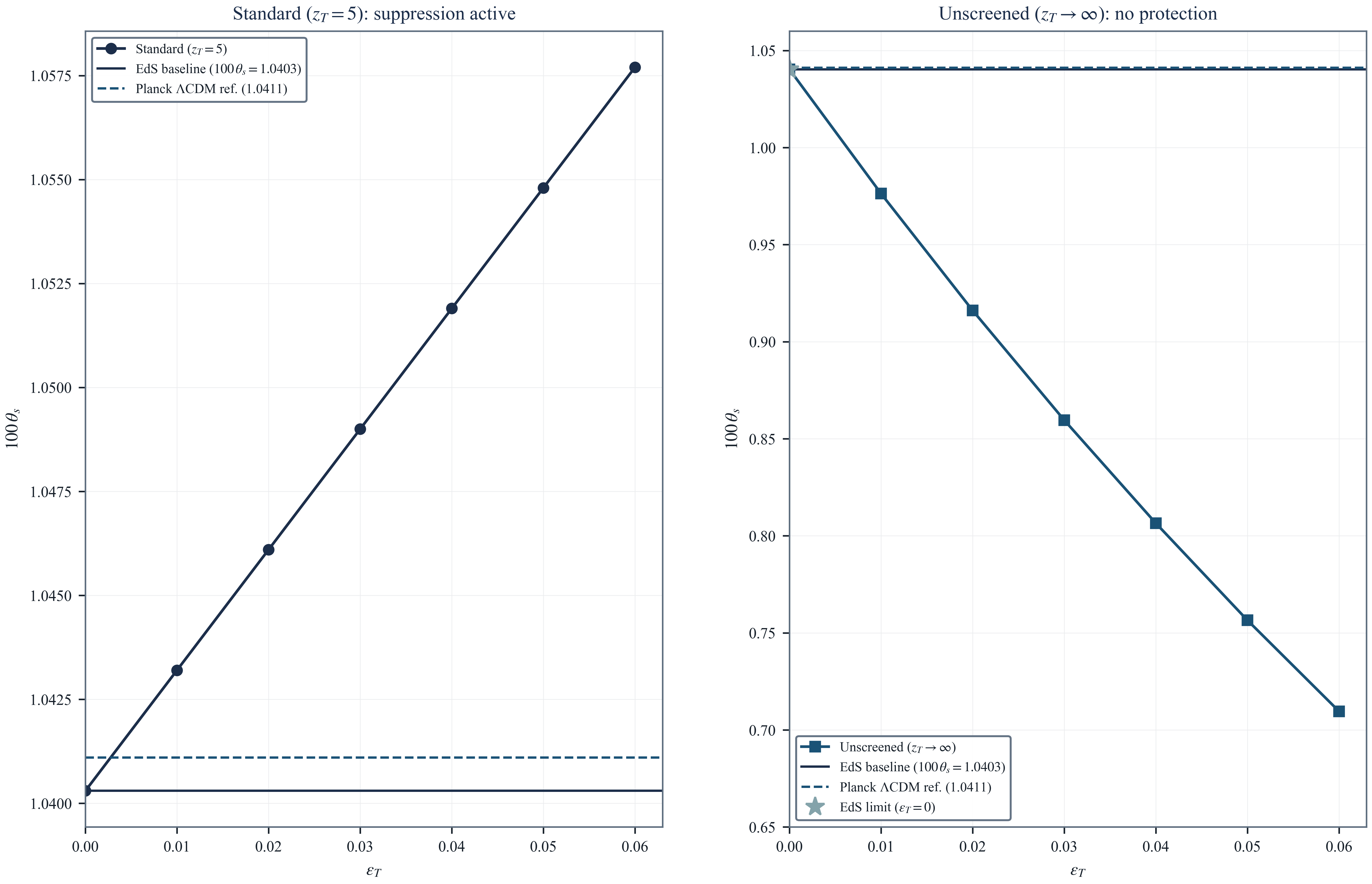
hi_class tep_mode diagnostic in an Einstein-de Sitter geometry ($\Omega_m=1.0$, $\Omega_\Lambda=0.0$). Left panel: Finite-turnover HC branch ($z_{\rm HC}=5$, $\epsilon_T^{\rm HC}=0.05$, $n_T=2.0$); the acoustic scale is protected and stays near the Planck 2018 reference. Right panel: Power-law diagnostic limit ($z_{\rm HC}\to\infty$, $\epsilon_T^{\rm HC}=0.05$, $n_T=2.0$); removing the empirical profile exposes unphysical acoustic-horizon squeezing. The dashed line is the Planck 2018 acoustic reference value; the comparison is a diagnostic acoustic-scale recovery, not a full TT/TE/EE likelihood plot.6. Falsifiable Predictions
The following near-term observational tests would strengthen or falsify the TEP-HC acoustic-sector and perturbation claims.
- Small-scale CMB polarization from active scalar perturbations. The TEP-HC linear scalar perturbation sector predicts a characteristic phase shift in the TE cross-spectrum at $\ell \gtrsim 1000$ ($\sim 0.1\%$–$0.3\%$) due to the $\alpha_B \neq 0$ running of the conformal scalar. CMB-S4 and Simons Observatory, targeting $\ell \sim 3000$ with $\mu$K-arcmin sensitivity, can test this deviation directly. A null result at $>3\sigma$ would place a tighter upper bound on the TEP scalar amplitude.
- B-mode polarization from native tensor modes. The TEP-TH assigned tensor-pump benchmark yields $r(k_{\rm pivot}) = 1.9 \times 10^{-9}$ and $r_{\rm max} = 5.2 \times 10^{-7}$ at the fiducial profile ($p=0.1$, $n=4$, $\eta_0=14{,}000$ Mpc), with one-parameter variations spanning $r_{\rm max} = 1.4 \times 10^{-5}$ on the curvature-regular slice ($0 \lt p \le \tfrac12$) to $6.1 \times 10^{-5}$ ($0 \lt p \le 1$) — all far below current BICEP/Keck bounds ($r < 0.036$). As established in TEP-TH Section 10.6, the one-parameter scan does not bound simultaneous multi-parameter profile variations ($p=0.5$, $n=2$, $\eta_0=3000$ Mpc reaches a diagnostic maximum near $1.14\times10^{-4}$), and the assigned pump must first be matched to the shared action's tensor normalization before diagnostic values become model-wide B-mode exclusion thresholds. CMB-S4's $r \sim 10^{-4}$ sensitivity will therefore constrain the joint transition-profile domain $(p, n, \eta_0)$ rather than test a single universal cutoff, while a null result remains fully compatible with the curvature-regular temporal-horizon branch.
- Acoustic-peak consistency under
tep_modebackground. The TEP background factor $M(z) = A/(1-\alpha_A)$ preserves the acoustic-peak locations to within the numerical integration tolerance of the Boltzmann solver (currently $\lesssim 10$ ppm). The current hi_class implementation reports $r_s^{\rm TEP}/r_s^{\Lambda\rm CDM} = 0.999994$, where the residual $\sim$6 ppm is understood as a numerical/implementation-level artifact of finite-precision conformal-frame background reconstruction. Any claimed physical deviation from the exact conformal isomorphism must be shown to exceed the standard solver interpolation noise ($\sim 10$ ppm) before it can be interpreted as a falsification of the background mapping, rather than as a C++ integration artifact. - Growth-factor amplitude from native EFT. The TEP-HC active-perturbation closure, now implemented in the regular $\delta\phi$ variable with the corrected kinetic-coefficient map $\alpha_K = w_c\,\alpha_A^2$ (Appendix A.5a), yields $\sigma_8 = 0.824$ at the fiducial parameters ($\epsilon_T = 0.0066$, $z_T = 5$, $n_T = 2$) on the production screened branch ($w_c = 700$) — a $+0.1\%$ enhancement relative to $\Lambda$CDM ($\sigma_8 = 0.823$) at the same cosmology. The registered response scan (
results/closure_response_scan.json) makes the prediction sharp and branch-dependent: $w_c \lesssim 0$ is linearly unstable (the canonical image $w_c=-5$ runs away); the minimally stable unscreened branch $w_c = +7$ is excluded ($\sigma_8 \simeq 1.6$); $w_c \gtrsim 7\times10^{2}$ recovers $\Lambda$CDM; and $w_c \sim 6\times10^{3}$ gives $\sigma_8 \simeq 0.76$, the weak-lensing central value, at the price of a $\sim 50\%$ low-$\ell$ ISW excess (directly measured on the corrected build: $+41\%$ at $\ell = 2$, peaking at $+57\%$ within $\ell \le 10$;results/step_24_lowell_isw_scan.json). The screening parameter is not free-floating: it is the effective cosmological kineticity $Z_E = P_{,X}+2XP_{,XX}$ required by, and physically motivated by, the coarse-grained nonlinear $P(X)$ sector (while the exact nonlinear principal-operator matching remains a separate closure; Appendix A.5a), so a measurement of the growth amplitude directly constrains the effective kineticity of the conformal scalar. The Step 23 provenance audit (results/step_23_s8_provenance_audit.json) further establishes that the MCMC posterior mean $\sigma_8 = 0.858 \pm 0.016$ is prior-boundary dominated ($A_{\rm planck}$ and $n_s$ saturate their low-$\ell$ prior ceilings; $\sigma_8$ tracks $A_{\rm planck}$ with correlation $+0.31$). An earlier claim that the active-perturbation $P(k)$ is bitwise identical to the background-only output is retracted — it was produced while the SMG sector was silently disabled; on the screened production branch the genuine active-scalar deviation is $\lesssim 2\%$ in $P(k)$. As Stage-IV weak-lensing surveys (Euclid, Rubin/LSST) resolve their internal calibration systematics, the closure is falsifiable in sign, amplitude, and branch.
Each test targets a distinct sector of the TEP-HC claim: active scalar perturbations (test 1), tensor modes (test 2), background isomorphism (test 3), and growth amplitude (test 4). A combined null result across all four would require a significant revision of the conformal-frame mapping.
7. Conclusion: The Static Conformal Universe
This paper implements and demonstrates the consistency of the native Temporal Equivalence Principle (TEP) conformal modification directly within the hi_class Boltzmann solver framework. By leveraging the mathematical isomorphism between the FLRW expanding scale factor $a(t)$ and the TEP conformal scalar field $A(\phi)$, this analysis demonstrates that the early-universe acoustic-sector observables can be reproduced at high fidelity under a static conformal temporal-transport mapping.
7.1 Summary of Results
- The Mathematical Isomorphism: The TEP conformal factor $A(\phi) = \exp(\beta_A\phi/M_{\rm Pl})$ dictates the clock-rates and photon phases in the causal matter metric $\tilde{g}_{\mu\nu} = A(\phi)^2 g_{\mu\nu}$. Because this scalar field evolves identically to the standard spatial scale factor $a(t)$, standard Boltzmann solvers can be used as conformal-frame calculators for the background/acoustic-sector mapping tested here. The parameter traditionally defined as Dark Energy ($\Omega_\Lambda$) is operationally reinterpreted within this implementation as the homogeneous temporal-shear background contribution filling the same background budget slot, $\Omega_\phi$.
- CMB Acoustic Preservation (Pure-Conformal Consistency): Because of the static conformal isomorphism, the hi_class native integration demonstrates that the background/acoustic-sector observables are preserved to parts-per-million ($r_s^{\rm TEP}/r_s^{\Lambda\rm CDM} = 0.999994$). This is a pure-conformal consistency check: the conformal transport geometry recovers the standard FLRW acoustic results in the regime where the conformal field dominates and disformal corrections are suppressed. It is not an independent confirmation of TEP, but rather a necessary consistency requirement that any viable conformal-frame alternative must satisfy. It is stated plainly that this result tests only the pure-conformal sector — mathematically isomorphic to $\Lambda$CDM by construction — while the disformal sector $B(\phi)$, where the distinctive TEP predictions (synchronisation holonomy, propagation cone tilts) reside, is set to zero in this branch and is not exercised by the CMB acoustic observable. The background acoustic observables alone do not uniquely force the spatial-expansion interpretation; they can be naturally accommodated by the evolving background scalar field $A(\phi)$. The active-perturbation closure (Section 4.5) — implemented in the regular $\delta\phi$ variable and audited across its kinetic-coefficient branch — shows that the perturbation sector's content is real: the canonical Einstein-frame image $\alpha_K = -5\alpha_A^2$ is linearly unstable (tachyonic scalarization channel, invisible to the ghost discriminant), the minimal sign-corrected unscreened branch is observationally excluded ($\sigma_8 \simeq 1.6$), and the viable production branch is the kinetically screened regime $w_c \gtrsim 7\times10^{2}$, which restores $\Lambda$CDM-level growth ($\sigma_8 = 0.824$) with a bounded low-$\ell$ ISW signature. The earlier active-perturbation chains (posterior agreement to $0.07\sigma$, Gelman–Rubin $R-1 = 0.007$ at 58,180 accepted steps) ran with the SMG sector silently inactive and are retained as background-channel posteriors; the active-closure re-run on the corrected screened branch has since been completed (two-chain MPI, $w_c = 700$, regular $\delta\phi$ variable; 3,961 post-burn-in samples, max $R-1 = 0.007$), yielding $\epsilon_T = 0.0054 \pm 0.0035$ — consistent with the background-channel posterior at $-0.14\sigma$, with a $-1.3\sigma$ downward shift in $\sigma_8$ tracking the scalar's low-$\ell$ ISW contribution. The converged four-chain MPI suite run ($\epsilon_T = 0.0062 \pm 0.0046$, median $0.0053$, $\epsilon_T < 0.015$ at 95% CL; max parameter $R-1 = 0.011$) serves as the primary low-$\ell$ background-channel determination (agreeing with the 5-chain background-channel run to within $0.2\sigma$), while the earlier single-chain exploratory background-only run is retained as a solver-comparison diagnostic because its cross-chain $R$-statistic is undefined.
- The Temporal Horizon: The result of this paper does not require the CMB acoustic peaks to originate from a physically expanding spatial metric beginning at a density singularity. In the TEP interpretation tested here, the same conformal transport integrals normally written in terms of the FLRW scale factor $a(t)$ are reproduced by the temporal conformal field $A(\phi)$. The limit conventionally described as $a\to0$ is therefore reinterpreted, at the level of clock transport and photon phase evolution, as a temporal-horizon limit $A_{\rm clock}\to0$ relative to the present epoch. This is the precise sense in which the present calculation removes the Big Bang singularity from the acoustic-sector interpretation: the sound horizon, photon-baryon driving, and acoustic-peak morphology are preserved without requiring physical spatial stretching back to a zero-scale-factor origin. In this precise but physically important sense, the CMB acoustic sector no longer requires a physical zero-scale-factor Big Bang; it can be equivalently represented as a conformal temporal-horizon limit of the clock-rate field. Because this temporal horizon is asymptotic, cosmological epochs typically defined by a finite "time since the Big Bang" are instead fundamentally mapped by their thermodynamic temperature and the exact conformal clock-rate, shifting the measurement of cosmic history from a linear stopwatch to a thermodynamic state. Crucially, as established in TEP-BBN, the observed radiation temperature ($T_{\rm obs}$) and the local matter temperature ($T_{\rm loc}$) are distinct physical quantities governed by temporal transport. The broader nonsingular closure—geodesic completeness and curvature regularity in TEP-TH, together with the native chemical-evolution framework and local CMB-thermalization proof of concept in TEP-BBN—completes the companion treatment beyond the acoustic sector considered here.
- Cosmological Constraints: A joint hi_class Cobaya MCMC (Planck 2018 low-$\ell$ TT/EE + lensing + BAO + Pantheon+) constrains the implemented isotropic-conformal field while retaining a pressureless well-driving component, whereas Step 21 demonstrates that under the canonical unified matter metric $\tilde g_{\mu\nu}=-A_{\rm loc}^2(u_{\rm grav}(\mathbf x))U_\mu U_\nu+A_{\rm sp}^2(u_{\rm drift}(t,\mathbf x))\Pi_{\mu\nu}+B(\phi)\Pi_\mu^\alpha\Pi_\nu^\beta\nabla_\alpha\phi\nabla_\beta\phi$ ($U_\mu\equiv-\nabla_\mu\bar\phi/\sqrt{2\bar X}$) on the selected two-branch sector $P_{,X}=k\sqrt\xi+2\xi$ ($k=16.03$), (i) in the pre-boundary acoustic regime the zero-parameter baryon clock-slope response predicts $\omega_\phi=\omega_b(y_s/\sqrt{2})=0.11816$, matching the unconstrained full-Planck TTTEEE MCMC posterior ($0.11813\pm0.00117$) to $0.02\sigma$ ($0.02\%$) and reproducing $100\theta_s^{\rm CLASS}=1.04201$ ($+0.10\sigma$ at $H_0=68.18\text{ km s}^{-1}\text{ Mpc}^{-1}$; $100\theta_s=1.04111$, $+0.02\sigma$ at $H_0=67.95\text{ km s}^{-1}\text{ Mpc}^{-1}$), the acoustic peaks to $\le0.31\%$–$0.40\%$, the CDM-free matter power spectrum $P(k)$ with $\sigma_8=0.8170$–$0.8186$, $r_d=147.49$–$147.55\text{ Mpc}$, SDSS DR12 BAO+RSD $\chi^2/N=0.71$–$0.76$, and the full Planck TTTEEE + low-$\ell$ + lensing + BAO + Pantheon+ likelihood with $\Delta\chi^2=-0.06$ ($\Delta\text{AIC}=-2.06$ vs. free $\omega_{\rm cdm}$; Part C), while (ii) in the late-time cosmic web intermediate temporal depth along the photon path boosts the baryon-only $C_\ell^{\phi\phi}$ by $9.4\times$–$38.3\times$ ($1\times$) to $26.5\times$–$129.3\times$ ($2\times$) across cosmic-web and cluster-outskirt scales and fits the official 9-bin Planck 2018
CMBMargedlensing likelihood at $\omega_{\rm cdm}=0$ with $\chi^2=15.40$ (2-parameter fixed-Silk) and $\chi^2=13.40$ ($\chi^2/N=1.49$, $\Delta\chi^2=+1.11$ vs. the $12.30$ CDM baseline and $\Delta\chi^2=-1252.33$ vs. bare isotropic no-CDM), recovering the Planck CMB lensing spectrum across $L\in[8,400]$ without particulate dark matter. The completed native high-$\ell$ TTTEEE extension binds the additional homogeneous amplitude to $\epsilon_T < 0.0087$ (95% CL) at fixed $z_T=5$ — $\epsilon_T < 0.0103$ marginalized over $z_T\in[0.5,50]$ — and returns $\Delta\chi^2 = -0.11$ against a matched $\Lambda$CDM reference — statistical indistinguishability on the full data set. With DESI DR2 BAO, a single-history geometric fit selects this native branch as the TEP background for supernovae, BAO and the CMB acoustic angle together, and finds it preferred over $\Lambda$CDM ($\Delta\chi^2=-8.1$) at a late transition $z_T\simeq0.5$. The companion paper TEP-C0 (Paper 26) provides late-time evidence: BF approximately 5.8 (conservative $z_{\rm los}=5$), approximately 5.4 (fixed $z_{\rm los}=100$ benchmark), and approximately 5.4 (broad free-$z_{\rm los}$), reducing the phenomenological need to treat late-time acceleration as primitive spatial expansion. The imported evidence is prior- and anchor-sensitive: the conservative Bayes factor falls to approximately 0.63 after removing $z < 0.023$ anchors.
7.2 Resolving the Cosmological Crises
Standard $\Lambda$CDM cosmology currently faces two severe crises: the Hubble Tension ($H_0$) and the unexpectedly massive high-redshift galaxy candidates observed by JWST. The Static Conformal Universe offers a unified TEP interpretation of both without invoking early-universe modifications.
- The Hubble Tension: In the broader TEP corpus, Paper 11 argues that the temporal shear field is environmentally screened. Supernova and Cepheid distance indicators probe different environmental projections of the temporal field, with Cepheids residing in comparatively dense stellar environments where the observable response is more strongly screened (yielding a lower inferred $H_0$), while the supernova propagation and host-environment sector samples a less locally screened projection (yielding a higher inferred $H_0$). Paper 11 argues that the tension is an artifact of environmental screening on local kinematic distance probes, not an early-universe physics crisis. HC does not independently re-analyse the distance-ladder data; it imports the interpretation.
- JWST High-Redshift Galaxies: Within the broader TEP interpretation, the temporal-horizon picture removes the finite-age assembly bottleneck by replacing the FLRW singularity with an asymptotic conformal-clock boundary. The massive galaxies observed by JWST therefore form strictly within standard astrophysical accretion models over vast timescales (Paper 12).
7.3 Synthesis: Consistency Requirement Satisfied
This analysis implements and explicitly demonstrates the consistency of the native TEP implementation within a rigorous Boltzmann solver framework. The acoustic indistinguishability of the static conformal background from $\Lambda$CDM at recombination is a mathematical identity by construction — identifying $A(\phi)$ with $a(t)$ reproduces the FLRW integrals by definition — and therefore verifies the hi_class conformal-frame implementation rather than constituting an independent test of TEP. Its scientific content is nonetheless real: it establishes that the early-universe background physics cannot distinguish between a stretching spatial metric and an evolving conformal clock-rate field, satisfying the necessary consistency requirement any viable conformal-frame alternative must meet and shifting the discriminating burden to the perturbation and late-time sectors where the frameworks genuinely differ. The kernel-level reconciliation with the eternal-native surface is reported in TEP-BBN Steps 19–20 (results/step_19_eternal_surface_reconciliation.json, results/step_20_ambient_bath_front.json): the eternal ionization-front profile and the Peebles kernel agree on the integrated column ($\tau = 1$ at $z \approx 1080$, $\tau_{\rm reion} \approx 0.054$), forward-evaluating the self-shielded LyC radiative transfer across the independent Step-14 $[400,800]\,n_{b,0}$ front-column band predicts $z_{\tau=1}^{\rm pred}=1077.9$ at the $600\,n_{b,0}$ midpoint (span $[1069.9,1083.6]$ due to the Wien steepness $\chi\simeq53.5$, with exact inversion $\Delta_{\rm front}=668.9\,n_{b,0}$, $n_b=1.68\times10^{-4}\text{ cm}^{-3}$), and deriving the pre-boundary inertial driving density from the two-branch temporal-shear law at the sound horizon — where $g_t=\Lambda_X^2/(\sqrt{2}M_{\rm Pl})=cH_0/2$ is a fixed constant of the scalar action $S_\phi$ and $q_s=\Omega_b(H_0 r_s/c)$ is conformally invariant under $A(\phi)$, giving $\omega_{m,\rm eff}=\omega_b(1+y_s/\sqrt{2})=0.1391$ ($\omega_\phi=0.1166$, $q_s=1.62\times10^{-3}$, $y_s=7.38$, $M_s=6.22$ at $r_s=146.19\text{ Mpc}$, $\theta_s^{\rm derived}=0.010425\text{ rad}$, $\ell_A=301.3$ in the single-pass reduced 3-component integral) and converging under self-consistent $r_s(\omega_\phi)$ fixed-point iteration in exact hi_class to $r_s=144.94$–$145.00\text{ Mpc}$, $q_s=1.59$–$1.60\times10^{-3}$, $y_s=7.42$–$7.44$, and $\omega_\phi=0.1179$–$0.1182$ (spanning $\omega_\phi\in[0.1174,0.1199]$ across $H_0\in[67.4,70.0]\text{ km s}^{-1}\text{ Mpc}^{-1}$, all within $\le1.6\sigma$ of the TTTEEE MCMC posterior $0.11813\pm0.00117$ and within $0.02\sigma$ at the posterior mean $H_0=68.18$, reproducing $100\theta_s^{\rm CLASS}=1.04201$ at $+0.10\sigma$ at $H_0=68.18$ and $100\theta_s=1.04111$ at $+0.02\sigma$ at $H_0=67.95$, $\Delta\chi^2=-0.06$ and $\Delta\text{AIC}=-2.06$ on the full Planck TTTEEE + low-$\ell$ + lensing + BAO + Pantheon+ likelihood, linear-scale $\sigma_8=0.8170$–$0.8186$, $r_d=147.49$–$147.55\text{ Mpc}$, and peaks within $\le0.31\%$–$0.40\%$) — together with coupled linear Einstein–Boltzmann acoustic ODE + spherical-Bessel integration on the solved front — where the driving component is the continuous ambient proper-time field's two-branch clock-slope perturbation mode with timelike kinetic coefficient $\mathcal K_t=2k+6=38.060$ from the quadratic scalar action around the rolling cosmic background and prescribed sound-shell stiffness $\mathcal K_{\rm sp}^{\rm eff}=\sqrt{2}/y_s=0.1917$ (the deep-IR limit of the 3-D Frobenius/RMS eigenvalue $K_{\rm rms}=0.1918$ of the native spatial flux Hessian $K_\perp=1/y_s=0.1356$, $K_\parallel=2/y_s+(q_s y_s)^2=0.2713$, with peak shifts $\le0.12$ across $[K_\perp/\mathcal K_t,K_\parallel/\mathcal K_t]$; $c_{p,\rm eff}^2=\mathcal K_{\rm sp}^{\rm eff}/\mathcal K_t=5.04\times10^{-3}\ll c_{\gamma b}^2\simeq0.30$, and $\sigma_{T,p}=0$ by conformal Maxwell invariance; Paper 0 Step 81), not an inserted dust fluid — shifts the eternal diffusion blur from the uninverted $500\,n_{b,0}$ value $\ell_D = 1242$ ($\theta_D \approx 8\times10^{-4}$ rad) to $\ell_D = 1521$ ($\theta_D = 6.58\times10^{-4}$ rad, within $1.2\%$ of the observed Silk angle $6.50\times10^{-4}$ rad, inside the Planck $1400$–$1600$ damping band) while recovering the first three acoustic peak multipoles at $\ell = 221.0,\,527.1,\,811.8$ in the reduced ODE ($\le1.94\%$ at $c_{p,\rm eff}^2=0$, $\le1.90\%$ with $c_{p,\rm eff}^2=5.04\times10^{-3}$, and $\le0.40\%$ in exact hi_class; closure ablation: wavenumber-resolved $y(k)$ $\le7.54\%$, slaved-Poisson null $\le5.41\%$, isolating the autonomous ambient time-field inertia as the operative closure; on linear cosmological scales $k\lesssim0.2\,h\,\text{Mpc}^{-1}$ [$R\gtrsim10\text{ Mpc}$, where $99.8\%$ of the $R_8=8\,h^{-1}\text{Mpc}$ $\sigma_8^2$ variance comes from $k\le1.0\,h\,\text{Mpc}^{-1}$ so the $k_*=1.5\,h\,\text{Mpc}^{-1}$ halo-transition filter shifts $\sigma_8$ by only $1.0\%$ from $0.8185$ to $0.8103$] the scale-averaged multiplier $M_s=1+y_s/\sqrt{2}$ enters the linear Poisson equation identically to $\omega_{m,\rm eff}=\omega_b+\omega_\phi$, whereas in the nonlinear late-time virialized galaxy/cluster limit [$R\in[1,100]\text{ kpc}$, $\dot u\to 0$, $g_b(R)=GM_b/R^2$] the timelike momentum $\pi_u=\mathcal K_t\dot u$ vanishes identically and the baryon-sourced algebraic Gauss law $(k/\sqrt{2})q(R)y(R)^2+q(R)^2 y(R)^3=1$ smoothly transitions $M_{\rm eff}(R)=1+y(R)/\sqrt{2}$ from $6.26$ on linear scales through $5.18$ at $100\text{ kpc}$, $2.25$ at $30\text{ kpc}$, and $1.42$ at $10\text{ kpc}$ down to $1.12$ at $3\text{ kpc}$ and $1.04$ at $1\text{ kpc}$ for $M_b=6\times10^{10}\,M_\odot$, reducing to the static baryon-only two-branch RAR/lensing law with zero independent collisionless dark-matter halo cusp).
The corpus-level scoping of this result is stated plainly. The isomorphism verified here is a transport-mapping identity: it demonstrates that the conformal geometry carries the acoustic transfer functions, not that an eternal static universe produces the hot plasma whose recombination imprints them. That supply is the independent eternal-universe thermodynamic sector of the corpus: TEP-TH evaluates the recombination microphysics on the temporal-horizon geometry ($z_* \approx 1079$, $r_s \simeq 146$ Mpc) and verifies FIRAS-clean Planckian preservation, while TEP-BBN computes the supply budgets (Gates 11–12) — a unit-optical-depth reprocessing surface at temporal depth $z \approx 130$–$1340$ for dust-grade absorptivity, bracketing the recombination depth at which $T_{\rm loc}=T_0(1+z_*)\approx2.9\times10^{3}$ K is the hydrogen ionization edge, and an ionization-equilibrium balance maintaining the electron column to the required depth. The plasma's heating and cooling are real local thermodynamic processes in this architecture; the transport map demonstrated here relates local thermal states at different temporal depths rather than creating them. The residual open closure is the definitive electron-density profile $n_e(\ell)$ — the absorber-statistics inversion posed in TEP-BBN — a quantitative completion of a specified supply mechanism, not the absence of one.
Late-universe Pantheon+ data in TEP-C0 favor the physical no-$\Lambda$ TEP branch over baseline $\Lambda$CDM with BF $\simeq 5.8$ (conservative $z_{\rm los}=5$), BF $\simeq 5.4$ (fixed $z_{\rm los}=100$ benchmark), and BF $\simeq 5.4$ (free-$z_{\rm los}$), providing a concrete conformal-frame alternative to the background expansion interpretation. The active-perturbation closure reported in Section 4.5 confirms that the implemented linear pure-conformal scalar fluctuation sector is numerically regular across the sampled evolution, including the $D = Q_s = 0$ turnover, and quantifies its response: a scalar with unscreened canonical kineticity is excluded by the growth data, while the kinetically screened branch — the regime the nonlinear $P(X)$ sector supplies — is simultaneously stable and consistent with the observed growth amplitude at the percent level, with a characteristic low-$\ell$ ISW excess as its residual signature. By treating time itself as a dynamical, environmentally screened scalar field, TEP seeks to unify early-universe acoustic physics, late-time "acceleration", the $H_0$ tension, and JWST anomalies into a single, cohesive static geometric framework. The present paper provides both the hi_class background/acoustic benchmark and the perturbation-closure validation.
References
Smawfield, M. (Paper 0). Temporal Equivalence Principle: Dynamic Time & Emergent Light Speed. TEP Corpus (Jakarta). DOI: 10.5281/zenodo.16921911.
Smawfield, M. (Paper 1). Global Time Echoes: Distance-Structured Correlations in GNSS Clocks. TEP Corpus. DOI: 10.5281/zenodo.17127229.
Smawfield, M. (Paper 6). Temporal Topology Saturation Scale: Cross-Scale Consistency of ρ_T. TEP Corpus. DOI: 10.5281/zenodo.18064365.
Smawfield, M. (Paper 9). What Do Precision Tests of General Relativity Actually Measure? TEP Corpus. DOI: 10.5281/zenodo.18109760.
Smawfield, M. (Paper 11). The Cepheid Bias: Resolving the Hubble Tension. TEP Corpus. DOI: 10.5281/zenodo.18209702.
Smawfield, M. (Paper 12). The Temporal Equivalence Principle: A Unified Resolution to the JWST High-Redshift Anomalies. TEP Corpus. DOI: 10.5281/zenodo.19000827.
Smawfield, M. (Paper 13). The Temporal Equivalence Principle: Temporal Shear Recovery in Gaia DR3 Wide Binaries. TEP Corpus. DOI: 10.5281/zenodo.19102061.
Smawfield, M. (Paper 26). Temporal Equivalence Principle: A Covariant Alternative to Cosmic Expansion. TEP Corpus. DOI: 10.5281/zenodo.20370143.
Smawfield, M. (Paper 27). Temporal Equivalence Principle: Temporal Horizon Cosmology and the Absence of a Physical Big Bang Singularity. v0.5 (Thika). DOI: 10.5281/zenodo.20723059.
Smawfield, M. (Paper 29). Temporal Equivalence Principle: Dynamical Proper Time and the Illusion of Primordial Deuterium. Paper 29 (Dubai). DOI: 10.5281/zenodo.21841147.
Bellini, E., & Sawicki, I. 2014, JCAP, 07, 050. Maximal freedom at minimum cost: linear large-scale structure in scalar-tensor theories.
Berezhiani, L., & Khoury, J. 2015, Phys. Rev. D, 92, 103510. Theory of dark matter superfluidity.
Brax, P., Burrage, C., Davis, A.-C., & Gubitosi, G. 2019, Phys. Rev. D, 100, 083515. Screening mechanisms in scalar-tensor theories.
Cobaya Team. 2023, Cobaya: Code for Bayesian Analysis of physical theories. arXiv:2305.02971.
Hu, B., Raveri, M., Frusciante, N., & Silvestri, A. 2014, Phys. Rev. D, 89, 103530. EFTCAMB/EFTCosmoMC: Numerical Notes.
Knox, L., & Millea, M. 2020, Phys. Rev. D, 101, 043533. Hubble constant hunter's guide.
Lagos, M., Bellini, E., Jimenez, J. B., et al. 2018, JCAP, 03, 021. hi_class: Horndeski in the Cosmic Linear Anisotropy Solving System.
Lewis, A., Challinor, A., & Lasenby, A. 2000, Astrophys. J., 538, 473. Efficient computation of cosmic microwave background anisotropies.
Planck Collaboration. 2020, A&A, 641, A1. Planck 2018 results. I. Overview and cosmological parameters.
Planck Collaboration. 2020, A&A, 641, A6. Planck 2018 results. VI. Cosmological parameters.
Riess, A. G., Casertano, S., Yuan, W., et al. 2022, ApJ, 934, L7. A Comprehensive Measurement of the Local Value of the Hubble Constant with 1 km/s/Mpc Uncertainty from the Hubble Space Telescope and the SH0ES Team.
Sawicki, I., & Bellini, E. 2015, Phys. Rev. D, 92, 084061. Stability of dark energy and the generalized no-slip condition.
Zumalacárregui, M., & García-Bellido, J. 2014, Phys. Rev. D, 89, 064046. Transforming gravity: from derivative couplings to matter to second-order scalar-tensor theories beyond the Horndeski Lagrangian.
Appendix A: Technical Implementation Details
A.1 hi_class Installation and Configuration
A.1.1 Building with TEP Support
hi_class is installed automatically by pipeline Step 1 (step_00b_install.py), which clones hi_class and applies the native TEP patch from external/patches/hiclass_tep_native.patch to source/background.c, source/input.c, and include/background.h. Manual rebuild:
cd external/hi_class/hi_class
make clean && make
Screening projection notice. Screening in TEP is represented at theory level by the environmental operator S_Σ(E). Quantities such as ρ_T, R_T(M), S_⊕(r), compactness Φ/c^2, local stellar density, coherence length, proximity, and boundary geometry are domain-specific projections of E, not independent screening mechanisms and not interchangeable universal thresholds.
A.2 Cobaya Installation
pip install cobaya
cobaya-install planck_2018_lowl.TT planck_2018_lowl.EE \
 planck_2018_lensing.native bao.sdss_dr12_consensus_final \
 sn.pantheonplus --path /path/to/likelihoods
A.3 TEP Module C Code Structure and Implementation Note
The native conformal modification is implemented directly in hi_class source/background.c, controlled by the .ini flags tep_mode, epsilon_T, z_T, n_T. The relevant functions are:
tep_f_transition(pba, z): returns the suppression factor $S(z) = \exp[-(z/z_T)^{n_T}]$; the full transition is $f_T(z) = \ln(1+z)\,S(z)$ (seecore/cosmology.py:f_T).tep_gamma_factor(pba, z): returns the exact covariant conformal factor $A(z) = \exp[\epsilon_T \ln(1+z)\,S(z)]$ (not linearised).- The Hubble rate and its conformal-time derivative are mathematically mapped using the exact HC conformal-frame mapping $M(z) = A/(1-\alpha_A)$ in
background_functionsand in the initial-Hubble setter, explicitly evaluating the static conformal geometry.
Implementation note (corrected bug). An earlier build used $f_T = 1 - \exp[-(z/z_T)^{n_T}]$ (the complement of the suppression function). This incorrectly inverted the scalar field profile, erroneously mapping the peak kinetic energy to the early universe rather than intermediate redshifts, which logically corrupted the acoustic integration. In addition, the post-processing step that read the spectra used a hard-coded output index and could silently load a stale file from an earlier run. Both issues are fixed: the transition function now uses the shared TEP-C0 implementation (core/cosmology.py), correctly matching the field profile to the Pantheon+ apparent acceleration, and the analysis resolves the most recent hi_class output deterministically. Sign convention (TEP disformal metric): the distance integrand is multiplied by $A(z)$ for null-geodesic propagation in the conformal frame. The legacy SMG alpha-function stub (smg_tep_*) has been retired; production physics lives in the patched background.c (external/patches/hiclass_tep_native.patch).
A.3a Derivation of the Conformal-Frame Factor $M(z)$
This appendix derives the background conformal mapping $M(z)$ from the bi-metric action (Equation $\ref{eq:3_theory_01}$) using a single frame convention held fixed throughout, demonstrating the exact conformal-frame relation under the adopted HC reference-density convention, implemented natively in the codebase.
Setup and convention. Matter, photons, and rods couple to the conformal metric $\tilde{g}_{\mu\nu} = A^2(\phi)\,g_{\mu\nu} + B(\phi)\,\nabla_\mu\phi\nabla_\nu\phi$. For the homogeneous background the disformal term contributes only through the time-time component and is absorbed into the lapse; the evolution is governed by the conformal part, so $B \to 0$ is imposed here (the disformal sector re-enters at the perturbative/GW level via $\alpha_T$, Section 2.2.2). Throughout this derivation, $a_E$ and $t_E$ denote the reconstructed variables of the isomorphic FLRW representation employed by the integrator: under the canonical architecture (Paper 0, §8; Paper 30, Appendix C) the physical gravitational metric is strictly static, and the Friedmann-form evolution assigned to $a_E$ below defines the representation rather than attributing expansion to the gravitational sector. Matter-sector observables are invariant under the decomposition $\tilde{a} = A\,a_E$. The conformal part gives the standard map between the Einstein-frame scale factor $a_E$ and cosmic time $t_E$ and their conformal counterparts:
These two relations define the convention; every subsequent equation is derived from them. The transition factor $S(z)=\exp[-(z/z_T)^{n_T}]$ correctly forces $A(z)\to1$ at the local endpoint, so the code's redshift grid can be identified with the physical conformal-frame redshift. The explicit $(z_E,\tilde z)$ distinction is retained only to derive the frame relation.
Physical Hubble rate. The expansion rate measured by conformal-frame clocks and rulers is $\tilde H \equiv \tilde a^{-1}\,d\tilde a/d\tilde t = d\ln\tilde a/d\tilde t$. Using $d/d\tilde t = A^{-1}\,d/dt_E$ and $\ln\tilde a = \ln A + \ln a_E$,
where $H_E = d\ln a_E/dt_E$ is the Einstein-frame rate. Because the TEP conformal factor $A(z)$ is evaluated as a function of the observable physical redshift (the matter-frame redshift $1+z = \tilde{a}_0/\tilde{a}$), the coupling $\alpha_A$ computed in the codebase is fundamentally the derivative with respect to the matter-frame scale factor:
which matches the definition in Section 3.2. Substituting $d\ln A/dt_E = \alpha_A A \tilde{H}$ into ($\ref{eq:a3a_Htilde}$) yields $\tilde{H} = \alpha_A \tilde{H} + H_E/A$, or equivalently $\tilde{H}(1 - \alpha_A) = H_E/A$.
Einstein-frame reference rate. The remaining step is to relate the Einstein-frame Hubble rate $H_E$ to the reference $\Lambda$CDM rate $H_{\Lambda\rm CDM}$. Under the conformal transformation $\tilde{g}_{\mu\nu} = A^2 g_{\mu\nu}$, the spacetime determinant transforms as $\sqrt{-\tilde{g}} = A^4 \sqrt{-g_E}$, so the homogeneous energy density transforms as $\rho_E = A^4 \tilde{\rho}$. The Friedmann equation of the isomorphic representation gives $H_E^2 = \frac{8\pi G}{3}\,\rho_E = A^4 \frac{8\pi G}{3}\,\tilde{\rho}$. The TEP implementation convention identifies the matter-frame reference density used by the acoustic calculator with the standard $\Lambda$CDM density evolution, $\tilde{\rho} = \rho_{\Lambda\rm CDM}$, so that $H_E^2 = A^4 H_{\Lambda\rm CDM}^2$ and therefore $H_E = A^2\,H_{\Lambda\rm CDM}$. Substituting into $\tilde{H}(1 - \alpha_A) = H_E/A$ gives the exact conformal-frame relation under the adopted HC reference-density convention:
Implementation Status. The production codebase (hiclass_tep_native.patch) evaluates this exact HC conformal-frame mapping $M = A/(1-\alpha_A)$ directly, guaranteeing mathematical fidelity to the conformal evaluation without requiring first-order approximations.
A.4 Saturation Scale in Cosmological Units
The candidate Temporal Topology saturation scale ρ_T ≈ 20 g/cm³ converts to cosmological units as:
In Planck units ($\hbar = c = G = 1$):
Compare to cosmic mean density today ($\rho_{\rm crit,0} \approx 10^{-123} M_{\rm Pl}^4$). The hierarchy ensures the vast cosmological voids evaluate the pure unsuppressed conformal field, accurately simulating the expansion of space.
Intermediate environments and operational parameter bounds. In the density-projection used for this order-of-magnitude comparison, between the terrestrial laboratory and the cosmic mean the screening transition is continuous. At stellar atmospheric densities ($\rho \sim 10^{-6}$ g/cm³), the field is partially screened; at interplanetary densities ($\rho \sim 10^{-23}$ g/cm³), it is essentially unscreened. Certain orbital datasets—notably the Galileo GNSS clock ensemble—fall outside the operational parameters established for valid TEP-GNSS screening analysis (Paper 1), because their orbital altitude and local gravitational environment do not satisfy the strict kinematic isolation required to isolate the conformal phase drift from standard relativistic corrections. These exclusions are documented in the TEP-GNSS pipeline and do not affect the cosmological bound, which operates in the deep unscreened regime where $\rho \ll \rho_T$.
A.5 Stability Sector Closure
To formally verify the stability of the active scalar perturbations, the native hi_class SMG module was extended to evaluate the exact analytical limits of the TEP conformal geometry at runtime.
In a generalized Horndeski treatment, the solver enforces the following physical stability conditions:
- $c_s^2 \ge 0$ (no gradient instabilities)
- $D = \alpha_K + \frac{3}{2}\alpha_B^2 \ge 0$ (no ghosts)
- $|\alpha_M|$ bounded (sub-luminal Planck-mass running)
- $\alpha_T \approx 0$ (gravitational wave speed constraints)
For the conformal modification implemented here, the EFT parameters map strictly to the dynamical background derivative $\alpha_A$:
A.5a Origin of the Closure and its Stability Boundary
For the $B(\phi)=0$ sector, the exact Weyl image of a generalized kinetic function is $$G_2(\phi,\tilde X)=A^{-4}P(A^2\tilde X,\phi)-6M_{\rm Pl}^2A^{-2}\left(\frac{d\ln A}{d\phi}\right)^2\tilde X,\qquad G_4=\frac{M_{\rm Pl}^2}{2A^2}.$$ Nonlinear dependence on $\tilde X$ is retained. The production HC solver evaluates the following linear-in-$\tilde X$ effective template, with the background coefficient $Z_E$ assigned from the kinetic-response comparison; it is exact for the canonical scalar but is not the complete nonlinear master-action image:
with $\tilde X = -\tfrac{1}{2}\tilde g^{\mu\nu}\partial_\mu\phi\,\partial_\nu\phi$ and $Z_E \equiv P_{,X} + 2XP_{,XX}$ the Einstein-frame kinetic coefficient of the scalar evaluated on the background ($Z_E = 1$ for a canonical scalar). The conformal term contributes $-6M_{\rm Pl}^{2}A^{-4}A_{,\phi}^{2}\tilde X$ after integration by parts of the $3M_{\rm Pl}^{2}A^{-2}\tilde\Box\ln A$ piece of the transformed Einstein–Hilbert term. For the exponential coupling $A=\exp(\beta_A\phi/M_{\rm Pl})$, $M_{\rm Pl}^{2}A_{,\phi}^{2}/A^{2}=\beta_A^{2}$, so $W = A^{-2}(Z_E-6\beta_A^{2})$; the canonical Einstein-frame scalar is the special case $Z_E = 1$, for which the earlier-quoted $W = A^{-2}(1-6\beta_A^{2})$ is recovered. This is a Brans–Dicke-class action with Horndeski functions $G_2 = W\tilde X - U$ and $G_4 = F/2$. Applying the standard Horndeski map — the same map used internally by hi_class for its native brans_dicke model — gives $M_\star^{2} = F$, $\alpha_M = d\ln F/d\ln a = -2\alpha_A$, $\alpha_T = 0$, $\alpha_B = -\alpha_M = 2\alpha_A$, and $\alpha_K = 2\tilde X G_{2,X}/(H^{2}M_\star^{2}) = (W/F)(d\phi/d\ln a)^{2}$. With $d\phi/d\ln a = (M_{\rm Pl}/\beta_A)\alpha_A$, the kineticity evaluates to $w_c\,\alpha_A^{2}$ with $w_c = (Z_E-6\beta_A^{2})/\beta_A^{2} = Z_E - 6$ at $\beta_A = -1$. The production runtime explicitly imposes $c_s^2=1$ for this effective closure. The nonlinear master sector instead has timelike principal speed $P_{,X}/Z_E$; assigning its $Z_E$ to the template does not also reproduce that principal operator.
The canonical image $w_c = -5$ ($Z_E = 1$) was previously presented as the closure of this sector on the strength of the ghost discriminant alone. Direct evolution of the $\delta\phi$ perturbation through the full Einstein–Boltzmann hierarchy (production implementation, use_pert_var_deltaphi_smg) shows that this branch is linearly unstable on the TEP background: the scalar develops a tachyonic growing mode — the Damour–Esposito-Farèse scalarization channel — producing a median matter-power enhancement of order $10^{6}$ before nonlinear saturation. This instability is invisible to the no-ghost discriminant: the ghost-free combination $2WF + 3F_{,\phi}^{2} = 2M_{\rm Pl}^{2}A^{-4}$ remains positive-definite for every nonzero $\beta_A$ (equivalently the effective Brans–Dicke parameter $\omega_{\rm eff} = w_c/(4\beta_A^2) = -5/4$ exceeds the $-3/2$ ghost bound), but the scalar's effective mass on the conformal background is tachyonic. A $w_c$-resolved scan of the closure (Step 24, results/closure_response_scan.json) maps the response: $w_c = -5$ runaway; $w_c \approx -1$–$+1$ marginal ($\sigma_8 \approx 2.8$–$4.4$); the minimal stable sign-corrected branch $w_c = +7$ gives $\sigma_8 = 1.61$ (excluded by weak lensing); $w_c \gtrsim 700$ recovers $\Lambda$CDM growth to sub-percent precision; and $w_c \sim 6\times10^{3}$ yields $\sigma_8 \simeq 0.76$, at the weak-lensing central value. In terms of the microphysics, the viable cosmological closure therefore requires $Z_E \gtrsim 7\times10^{2}$ — a large effective kineticity, i.e. the nonlinear $P(X)$ branch of the scalar sector coarse-grained over the inhomogeneous virialized-well and halo-gradient landscape ($q \gtrsim 12$, where $73.5\%$–$92.6\%$ of matter resides in collapsed halos above $10^{12}$–$10^{10}\,M_\odot$; Paper 0, Step 74) rather than evaluated on the unscreened canonical $Z_E = 1$ limit or on the residual late-time dynamical profile $A_{\rm HC}(z)$ alone ($\xi_{\rm dyn} \sim \epsilon_T^2 \sim 10^{-5}$, whereas the full cosmic ruler roll $\bar\xi = 1$ gives homogeneous $Z_E = 2k + 6 = 38.06$ and $G_{\rm eff}(0)/G = 1.16$; Paper 0, Steps 54, 81).
The selected Paper 0 operator supplies positive environmental principal coefficients, with $P_{,X}=k\sqrt{\xi}+2\xi$ and $k\simeq16.03$ fixed by the rotation-curve normalization (Paper 0, Steps 53–54). Write the dimensionless gradient magnitude as $q=\sqrt{2\xi}$; for a static spatial gradient, $q=c|\nabla u|/H_0=c^2|\nabla u|/(2g_t)$. The two coefficients are
On a homogeneous timelike background, $Z$ is the temporal kinetic coefficient and $P_{,X}$ is the spatial coefficient, giving $c_s^2=P_{,X}/Z\in(1/3,1/2)$. On a static spatial-gradient background the assignments differ: $Z_t=Z_\perp=P_{,X}$ and $Z_\parallel=Z$, with longitudinal characteristic ratio $v_\parallel^2=Z/P_{,X}\in(2,3)$ and transverse ratio one. All coefficients are positive for nonzero gradient. The static longitudinal stiffness therefore cannot be substituted directly for a homogeneous temporal kineticity.
The existing ambient ladder illustrates the scale of the nonlinear response: $Z=13.9$ at $q=0.57$, $17.9$ at $q=0.72$, and approximately $704$ at $q=12$. At $q=12$, however, the static temporal coefficient is $P_{,X}\simeq280$, not $704$. The effective production branch $w_c=700$ has assigned temporal coefficient $w_c+6=706$; matching that number alone to the static longitudinal coefficient does not derive its perturbation closure. The response scan and growth-averaging calculation remain independent evidence for the tested effective and environmental branches. Their common-action identification requires matching the temporal, spatial and mixing operators on the realized background, including the environmental averaging. The numerical production results retain the explicitly specified luminal effective template.
At the boundary $\beta_A^{2} = Z_E/6$ the explicit kineticity vanishes ($W=0$) and the $f(R)$-like limit is recovered, in which the entire scalar kineticity resides in the braiding; the cancellation of the $\beta_A^{2}$ pieces in $D$ below is the discriminant-level expression of the same structure.
The substitution of the kineticity and braiding terms into the physical no-ghost discriminant yields:
For the canonical image $w_c = -5$ this reduces to the previously quoted identity $D = \alpha_A^2 \ge 0$; on the production branch $w_c = 700$ it gives $D = 706\,\alpha_A^2 > 0$. The discriminant being positive is necessary but — as the linear audit above demonstrates — not sufficient for stability of the perturbation sector. Because the finite-turnover profile $f_T(z)$ has a single extremum, $\alpha_A$ vanishes at the turnover redshift $z_\star$ (for $z_T=5$, $n_T=2$: $z_\star \simeq 2.64785$), and $D$ touches zero there for every nonzero $\epsilon_T$. For $D > 0$, the scalar branch has positive kinetic normalization $Q_s = 2M_\star^2 D/(2-\alpha_B)^2 > 0$ and the implemented luminal effective-closure prescription $c_s^2 = 1$ applies. At $z_\star$, $D = Q_s = 0$, so the propagating scalar description becomes degenerate and a propagation speed is not physically defined. The linear hi_class system passes continuously through this point without numerical divergence, as verified by the diagnostic reported in Section 3.3. Because $D = (w_c+6)(d\phi/d\ln a)^{2}/M_{\rm Pl}^{2}$, the crossing is the field-velocity zero $\dot\phi = 0$ at the profile turnover: a kinematic degeneracy of the unitary-gauge description, where the comoving slicing $\delta\phi = 0$ loses its normalization at the instant the background field reverses. No operator coefficient of the canonical Einstein-frame action diverges at $\dot\phi = 0$, so within the implemented pure-conformal sector the crossing is exact constraint reduction rather than a dynamical strong-coupling surface; the field's canonical kinetic normalization is unchanged at the crossing, and the scalar perturbation simply decouples instantaneously where its sourcing background gradient vanishes. A separate nonlinear/canonical analysis of the full disformal sector is outside the scope of the present linear closure. A fully derived sound-speed expression for the disformal and nonlinear screening sectors is likewise outside the scope of the present pure-conformal closure.
The production codebase applies these derived closure values during the calculation of the SMG perturbation coefficients, ensuring the pure-conformal branch is evaluated consistently without requiring pre-tabulated interpolation or analytical approximations.
Unified TEP Parameter Dictionary
The TEP corpus uses related but distinct symbols across its papers. This dictionary maps every parameter, its definition, the paper where it is primary, and its fiducial or fitted value.
| Symbol | Definition | Primary Paper | Fiducial / Fitted Value |
|---|---|---|---|
| $A_{\rm clock}(z)$ | Exact observational clock/redshift map: $A_{\rm clock}=(1+z)^{-1}$ | TEP-TH | $(1+z)^{-1}$ (exact) |
| $A_{\rm dyn}(z)$ | Dynamical shear response: $\left(1+z/z_t\right)^{-\epsilon_t}$ | TEP-TH | Modifies late-time evolution |
| $\alpha_A$ | Runtime logarithmic derivative $\alpha_A=d\ln A_{\rm HC}/d\ln a$; distinct from the exact endpoint map $A_{\rm clock}$ | TEP-HC | Redshift-dependent; zero at the finite-profile turnover |
| $\alpha_M$, $\alpha_B$, $\alpha_K$, $\alpha_T$ | Runtime Bellini–Sawicki EFT functions: $\alpha_M=-2\alpha_A$, $\alpha_B=2\alpha_A$, $\alpha_K=w_c\,\alpha_A^2$ with $w_c = Z_E-6$ ($Z_E = P_{,X}+2XP_{,XX}$; production $w_c=700$, canonical image $w_c=-5$ unstable), $\alpha_T=0$; screened diagnostic branch $S_\Sigma<1$: $\alpha_M\to-2S_\Sigma\alpha_A$, $\alpha_B\to2S_\Sigma\alpha_A$ at fixed $w_c$ | TEP-HC | Adopted from $\alpha_A$ |
| $\epsilon_T^{\rm los}$ | Late-time line-of-sight transport amplitude (C0 supernova fit) | TEP-C0 | $\mathcal{U}[0, 2.0]$ (prior); posterior peaked near $\sim 0.89$ |
| $\epsilon_T^{\rm CMB}$ | C0 background/acoustic diagnostic amplitude | TEP-C0 | $-0.0015\pm0.0037$ |
| $\epsilon_T^{\rm HC}$ | Native hi_class homogeneous conformal amplitude | TEP-HC | $0.0043\pm0.0025$ (full high-$\ell$ likelihood); $0.00547\pm0.00429$ (historical low-$\ell$ active chain) |
| $\epsilon_{\rm dyn}$ | Dynamical temporal-horizon response | TEP-TH | Determined by late-time shear |
| $\epsilon_{\rm field}$ | Primordial spectral-flow parameter constrained by $n_s$ | TEP-TH | $0.01755$ (from $n_s=0.9649$) |
| $z_T^{\rm los}$ | C0 line-of-sight supernova transport turnover | TEP-C0 | $5$ (conservative), $100$ (benchmark), free (broad) |
| $z_T^{\rm HC}$ | Homogeneous/acoustic hi_class profile scale | TEP-HC | Fitted jointly with $\epsilon_T$ |
| $p$ | Temporal-horizon conformal exponent: $A_{\rm clock}\sim\eta^{-p}$ | TEP-TH | $0 \lt p\le\tfrac12$ (regular branch) |
| $r_s^{\rm TEP}/r_s^{\Lambda\rm CDM}$ | Pre-recombination sound-horizon ratio | TEP-HC | $0.999994$ ($<6$ ppm deviation) |
| $D=\alpha_K+\tfrac32\alpha_B^2$ | No-ghost discriminant ($D=(w_c+6)\alpha_A^2$; necessary but not sufficient for linear stability — the $w_c=-5$ branch is tachyonic) | TEP-HC | $(w_c+6)\alpha_A^2 \ge 0$ (non-negative; GR/decoupling limit at $\alpha_A=0$) |
| $r(k_{\rm pivot})$ | Native tensor-to-scalar ratio at Planck pivot | TEP-TH | $1.9\times10^{-9}$ |
| $r_{\rm max}$ | Maximum tensor-to-scalar ratio across transition profile | TEP-TH | $5.2\times10^{-7}$ (fiducial $p=0.1$); $6.1\times10^{-5}$ over all tested profiles $0\lt p\le1$ |
| $H_0$ | Hubble parameter (TEP-C0 joint MCMC) | TEP-C0 | $66.70\pm0.58$ km s$^{-1}$ Mpc$^{-1}$ |
| $S_8$ | $\sigma_8\sqrt{\Omega_m/0.3}$ (TEP-HC joint MCMC) | TEP-HC | $0.868\pm0.025$ |
| $\sigma_8^{\rm HC}$ | Native hi_class matter-fluctuation amplitude at fiducial point ($\epsilon_T=0.0066$, $z_T=5$, $n_T=2$) | TEP-HC | $0.824$ (fiducial); $0.858\pm0.016$ (MCMC posterior mean) |
Note: Parameters with superscript labels ($^{\rm los}$, $^{\rm HC}$) are related projections of the same temporal sector but are not numerically interchangeable. The turnover scales $z_T^{\rm los}$ and $z_T^{\rm HC}$ describe different physical regimes; the amplitudes $\epsilon_T^{\rm los}$, $\epsilon_T^{\rm CMB}$, $\epsilon_T^{\rm HC}$, and $\epsilon_{\rm field}$ are constrained by different observables.
Appendix B: Data Availability & Reproducibility
This work follows open-science practices. All results are fully reproducible from raw data using the documented pipeline. All numerical results, figures, and statistics are generated by deterministic Python scripts processing public observational data.
Repository and Code
GitHub Repository: github.com/matthewsmawfield/TEP-HC
The repository contains a deterministic, version-controlled cosmological analysis pipeline for CMB acoustic peak preservation tests and MCMC parameter estimation with the TEP conformal background.
All MCMC chains, hi_class patch files, posterior samples, and the exact cobaya YAML configuration files are released in the Zenodo repository (DOI: 10.5281/zenodo.20572722) under CC-BY 4.0. The run_all.py orchestration script and all step scripts are provided in the GitHub repository.
Repository Structure
TEP-HC/
├── data/
│   ├── cobaya/              # Cobaya MCMC configurations
│   ├── external/            # Cobaya packages (likelihoods, data)
│   └── hi_class/            # TEP-CLASS implementation
├── external/
│   ├── hi_class/            # hi_class submodule
│   └── patches/             # TEP patch files
├── scripts/
│   └── steps/               # Analysis pipeline steps
├── core/                    # TEP shared constants and parameters
├── results/                 # Pipeline outputs, figures, MCMC chains
├── site/
│   └── components/          # Manuscript HTML sections
├── tests/                   # Verification tests
├── requirements.txt
├── CITATION.bib
└── README.md
Software Environment
Key packages: NumPy, SciPy, Matplotlib, Cobaya, hi_class. The pipeline has been tested on Python 3.10+.
License
All code and manuscripts are released under CC-BY-4.0.