
Abstract
Cosmological redshift is standardly interpreted as a geometric signature of spatial expansion. This interpretation requires a fundamental assumption that is defined herein as the Isochrony Axiom: the premise that, after gravitational and kinematic effects derived from the spacetime metric have been included, the calibration of every matter clock is fully exhausted by that single metric, so that no independently dynamical field may rescale matter proper time across cosmological epochs. Standard single-metric cosmology closed the temporal sector before the redshift was interpreted. In this paper, it is demonstrated that when matter-clock calibration is permitted an independent dynamical scalar degree of freedom ($\phi$), the measured cosmological redshift ($z$) can be rigorously derived from the ratio of matter-clock calibrations between emission and observation on a static spatial manifold. The scalar field defines a spatiotemporal clock geometry—the Temporal Topology—whose homogeneous evolution governs cosmological calibration and whose inhomogeneous disformal connection can become non-integrable, producing synchronization holonomy. Using the canonical matter metric of the Temporal Equivalence Principle (TEP), $\tilde g_{\mu\nu} = A^2(\phi)\,g_{\mu\nu} + B(\phi)\,\nabla_\mu\phi\,\nabla_\nu\phi$, the Mount Wilson Equivalence Theorem is proven: on a homogeneous, spatially flat, static gravitational background, with universal matter coupling and $A^2 - B\dot\phi^2 > 0$, the endpoint redshift $1+z = A_0/A_{\rm em}$ is observationally degenerate with the FLRW relation $1+z = a_0/a_{\rm em}$ at the level of the redshift observable alone. TEP is distinguished from a mere conformal rewriting by its separate matter and gravitational propagation sectors, making multi-messenger observations a principal inter-sector discriminator. The historical data from Mount Wilson Observatory are re-examined to separate the documented spectral displacements from the subsequent spatial inferences, demonstrating that the observed dynamics are consistent with a temporal reinterpretation on a static spatial manifold. Precision GNSS chronometry, pulsar scintillation, and Lunar Laser Ranging are identified as the empirical instruments capable of testing the temporal sector locally. Consequently, a globally consistent framework for an eternal, deterministic continuum is presented, supplying the common mathematical resolution to the questions that Einstein separated.
Keywords: cosmological redshift, isochrony axiom, scalar-tensor theory, static universe, temporal equivalence principle, expansion degeneracy, synchronization holonomy
Prologue: The Photograph
On 29 January 1931, Albert Einstein bent to the eyepiece of Mount Wilson's 100-inch Hooker telescope. Edwin Hubble and Walter Adams were present, members of the observational programme whose measurements appeared to show that the universe itself was expanding. The telescope revealed the cosmological spectral displacement; the geometry assigned to that displacement remained a theoretical inference. The photograph records the moment when the architect of relativistic spacetime confronted the instrument that had transformed a theoretical possibility into the dominant picture of the cosmos.
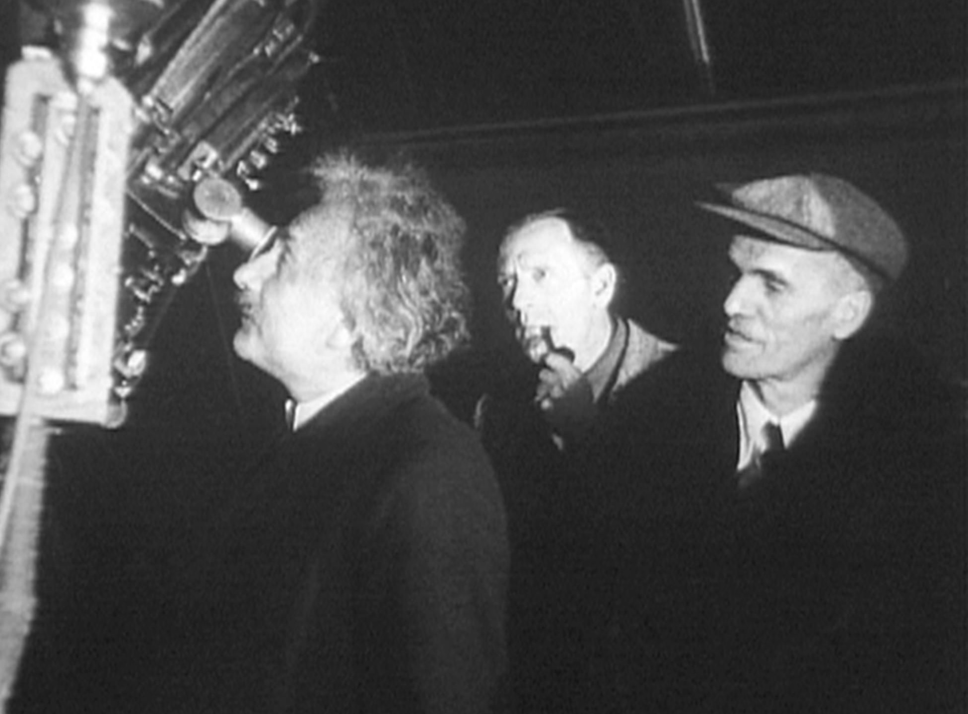
Einstein's encounter with Mount Wilson had begun long before Hubble's redshift programme. In 1913, he wrote to the observatory's founder, George Ellery Hale, asking whether stars close to the Sun could be observed in daylight, a possible test of gravity's effect on light 21. Eighteen years later, he returned to the same mountain, visiting both the 150-foot solar tower and the 100-inch Hooker telescope, to confront a still larger question: what could light reveal about the geometry of the universe?
The Hooker telescope was at the time the largest optical instrument in the world. It was here that Milton Humason and Edwin Hubble had recently assembled the data that would permanently alter the foundations of physics. Einstein encountered the observational results of the Mount Wilson programme, including the spectrographic measurements that showed unmistakable displacements of the calcium absorption lines toward longer wavelengths.
His visit is widely recorded as the moment he abandoned his 1917 model of a static, globally Machian universe 6. Confronted with a linear relationship between estimated distance and spectral redshift, Einstein accepted the dynamical geometry formulated by Georges Lemaître 12 and Aleksandr Friedmann 13. The universe was expanding, and the static cosmos was set aside as an incomplete theoretical closure. Einstein arrived in Pasadena amid extraordinary public attention: reporters, photographers, Hollywood figures, and enthusiastic hosts followed his movements. He was accompanied by his wife Elsa and his mathematical assistant Walther Mayer, the Viennese topologist known informally as "Einstein's calculator," who had been engaged specifically to work on the distant-parallelism programme 57. During a tour of the Mount Wilson facilities, Elsa was shown the great telescope and told that one of its chief purposes was to determine the shape of the universe. She reportedly replied: "My husband does that on the back of an envelope" 58. The anecdote captures the asymmetry of the moment: the most powerful spatial instrument in history, operated by men who had no chronometric machinery at all. To a New York Times reporter, Einstein described the experience in dramatic terms: "The redshift of distant nebulae has smashed my old construction like a hammer blow," he said, swinging down his hand to illustrate. Then he added: "The red shift is still a mystery" 64. The first statement entered the standard narrative. The second did not. Writing to his sister shortly afterward, Einstein remarked that he would soon "no longer have to play the part of the good Lord or his assistant" 53. That public spectacle formed the backdrop to a scientific transition that had nevertheless been developing for years.
This historical pivot established the conceptual foundation of the standard cosmological model. The Hooker telescope was an instrument of unprecedented spatial resolution, yet it operated in a state of what this paper terms Chronometric Blindness. It could measure the frequency of light to extraordinary precision; it possessed no mechanism for interrogating the independent dynamics of the proper time that governed the clocks of distant matter. The photographic plates captured the displaced frequencies of incoming photons. They did not directly record expanding space. What, exactly, did the telescope prove?
1. The Evidence
The transformation occurred with extraordinary speed. In April 1920, Harlow Shapley and Heber Curtis debated the scale of the Milky Way and the nature of the spiral nebulae 36. Eleven years later, Einstein stood at Mount Wilson confronting the claim that the entire spatial universe was evolving. Cosmology had passed from uncertainty about the existence of other galaxies to a theory of expanding space in little more than a decade.
The conclusion was not arbitrary. It arose from a formidable synthesis of observational astronomy, and reconstructing the chain of evidence that produced it is necessary to understand the transition of the 1930s.
Mount Wilson had transformed the universe once before. On a glass plate exposed on the night of 5-6 October 1923, Hubble identified a variable star in Andromeda. He crossed out his original mark for a nova and wrote, in emphatic letters, "VAR!" Leavitt's period-luminosity relation then placed Andromeda far beyond the Milky Way. A handwritten word on a small glass plate had enlarged the known universe. Six years later, another set of marks on other plates would be interpreted as showing that this larger universe was itself expanding.
The initial anomaly had emerged earlier, when Vesto Slipher measured the spectra of spiral nebulae 37. By 1917, he had found that twenty-one of twenty-five measured nebulae were redshifted. Twenty of the twenty-four velocities used in Hubble's famous 1929 diagram came from Slipher's work. Hubble's contribution was principally to connect those velocities with estimated distances. The famous diagram was not the product of one observer. Its velocity axis was built largely from Slipher's spectra; its distance scale depended on Leavitt's stellar periods; Hubble assembled the relation; and Humason extended it into the deeper universe. Modern cosmology emerged not from a single decisive observation but from the alignment of several different measurements under a common interpretation.
Nor did Hubble approach the data in an interpretive vacuum. Carl Wirtz 42, Knut Lundmark, and Gustaf Strömberg had already searched for relations between spectral displacement and distance, often under the influence of de Sitter's cosmology. The crucial question was therefore never simply whether a pattern existed. It was which theoretical language should be used to describe it.
The distance scale had an unexpectedly temporal foundation. Henrietta Leavitt compared the changing brightness of twenty-five variable stars in the Small Magellanic Cloud 38. Because those stars lay at approximately the same distance, she recognized that their periods revealed their intrinsic luminosities. Hubble's distance axis was therefore constructed from a stellar clock: the measured rhythm of a pulsating star. Time was already hidden inside the diagram that would later be interpreted as the expansion of space.
Humason's measurements were acts of extraordinary patience. A former mule driver and observatory janitor with little formal education, he became one of the finest spectroscopists of his generation. His two plates of NGC 7619 required exposures of thirty-three and forty-five hours 43. Across several nights, the telescope gathered enough light to reveal a few displaced absorption lines. The 100-inch mirror itself was a source of constant anxiety: the massive glass disk was sensitive to thermal gradients, and Hale had proposed refrigerating the entire dome to prevent the mirror from heating up during the day, though only a sunscreen was ultimately installed 54. The observers mastered temperature-dependent distortions in the glass because those distortions were measurable. A cosmological variation in matter-clock calibration lay outside the variables their framework permitted. The Chronometric Blindness was not confined to Mount Wilson. Across the 1920s and 1930s, astronomers including J. K. Fotheringham and John Jackson were documenting anomalous "accelerations" of the Sun and Moon against Greenwich Mean Time 69. The Moon appeared to be drifting ahead of its predicted ephemeris. The anomaly was real, but its interpretation was inverted: the celestial bodies were not accelerating; the Earth's rotation was slowing due to tidal friction. Spencer Jones confirmed this in 1939 70, but the concept of a time standard independent of Earth's rotation, Ephemeris Time, was proposed in 1948, adopted by the International Astronomical Union in 1952, and not introduced into official astronomical ephemerides until 1960 72. Throughout the entire Mount Wilson era, time was defined by the rotation of a single planet, and its irregularities were being misattributed to the dynamics of distant bodies. The global astronomical community had no framework for treating time itself as a variable physical quantity. A cosmological variation in the rate of proper time was not merely undetectable; it was conceptually inaccessible.
What emerged on the glass was not an image of a galaxy moving through space. It was a measurable displacement in the frequency of its light. The 1929 relation 1 drew on numerous previously published velocities, with Humason contributing several recent measurements. He subsequently undertook the arduous task of extending the spectrographic measurements to much fainter and more distant galaxies, culminating in the major 1931 Hubble-Humason paper 2 that extended the relation far beyond the original sample. The combined programme established that extragalactic redshift increased linearly with estimated distance.
In the theoretical domain, general relativity had already established that the metric tensor of spacetime ($g_{\mu\nu}$) was a dynamical entity. Willem de Sitter 16 had introduced a cosmological solution that, though presented in static coordinates, contained the seed of an expanding interpretation that would later be recognized through coordinate transformations by Lemaître and others. Aleksandr Friedmann 13 and Georges Lemaître 12 then explicitly demonstrated that Einstein's field equations permitted, and in most cases required, the spatial metric to evolve over time. The expanding interpretation did not originate on a photographic plate. By 1927, Lemaître had already brought the dynamical solutions of Einstein's equations into contact with the available redshift and distance estimates, deriving the velocity-distance relation and estimating the expansion rate two years before Hubble's 1929 paper. He sent a reprint to Eddington, his former supervisor, who filed it away and did nothing. The paper sat unnoticed for three years. It was not until the January 1930 meeting of the Royal Astronomical Society, where de Sitter presented the observational velocity-distance relation and both he and Eddington struggled to explain it theoretically, that Lemaître read the published report and wrote to remind Eddington of the forgotten paper. Eddington immediately recognized its significance, arranged for its English translation and publication in the Monthly Notices 56, and brought it to the attention of the international community. A further complication has recently emerged: the 1931 English translation omitted the key paragraphs in which Lemaître described the velocity-distance law and derived the expansion rate, replacing them with a single sentence quoting the adopted value 65. Lemaître himself edited the translation and voluntarily omitted his earlier numerical discussion, judging it superseded by Hubble's more recent results. In doing so, he surrendered the published evidence of his priority, and observational credit shifted almost entirely to Mount Wilson. The expanding universe was not born from a sudden empirical revelation on a Mount Wilson plate. It was retrieved from a desk drawer as a mathematically ready framework for theorists confronting an unexplained empirical relation.
When the Mount Wilson relation appeared, a mathematical interpretation was already waiting for it. Theorists immediately recognized a synthesis: the observed redshift could be elegantly explained as the continuous stretching of the spatial scale factor ($a(t)$) during the photon's transit from emitter to observer.
Confronted with this powerful relationship, the abandonment of the static universe appeared entirely rational. The observational evidence was robust, and the expanding spatial geometry provided a mathematically consistent mechanism to encompass it. ΛCDM may therefore be understood as an architecture constructed after the temporal sector had already been closed. Dark matter, dark energy, and inflation were developed within that architecture. The question is whether the original closure itself was ever independently tested.
Seen operationally, the Mount Wilson diagram was stranger than its familiar labels suggest. The telescope measured wavelength shifts, which were subsequently expressed as velocities; the distance scale was anchored by periodic stars, whose luminosities were inferred from their rhythms. One axis began as a frequency ratio, while the other was calibrated through a stellar clock. The diagram became a picture of spatial expansion only after these chronometric observables had been interpreted geometrically.
2. The Interpretation
The standard historical narrative often conflates the observational discovery with its physical interpretation. The two must be formally separated:
Operational Distinction. Spectral displacement is not a direct measurement of spatial expansion.
The first is a measured physical observable. The second is an inference drawn within the constraints of a specific theoretical framework. Spatial expansion was not recorded directly on the photographic plates; it was the chosen physical interpretation of the observed spectral displacement.
The primary astronomers of the era were acutely aware of this distinction. In 1929 Hubble described the quantities as "apparent radial velocities" and the paper itself is notably restrained in its cosmological interpretation, presenting the empirical relation without elaborating on its physical significance 1. In 1931, Hubble wrote directly to Willem de Sitter, explicitly disclaiming interpretive authority over his own data: "We use the term 'apparent' velocities to emphasize the empirical features of the correlation. The interpretation, we feel, should be left to you and the very few others who are competent to discuss the matter with authority" 60. His 1936 book, The Realm of the Nebulae 4, was predominantly observational in character; Hubble described himself as "primarily an observer" and confined theoretical interpretation to a brief concluding discussion. The 1936 Rhodes Lectures at Oxford, published as The Observational Approach to Cosmology 5, concluded that "a static universe with a hitherto unsuspected dependence of light frequency on distance is probably more acceptable than one or other of the homogeneous expanding models of general relativity," as reported in a contemporary Nature review 67. His explicit treatment of recession and an unknown non-kinematic mechanism as parallel possibilities emerged in his later work with Tolman 3 and in his 1936-1937 lectures 4,5.
This caution persisted throughout his career. In the 1935 study with Richard Tolman 3, Hubble attempted to distinguish between actual recession and a non-kinematic redshift using surface-brightness scaling, a test whose theoretical framework Tolman had developed in his treatise on relativity and cosmology 17. In an expanding universe, the Tolman prediction is a surface-brightness dimming proportional to $(1+z)^4$. In the simple stationary energy-loss model used for comparison, only one factor of $(1+z)$ appears. The 1935 data were insufficient to decisively distinguish the two predictions, a conclusion Hubble and Tolman stated explicitly. Later analyses by Lubin and Sandage 71 measured surface-brightness exponents below four and interpreted the shortfall as luminosity evolution; after that correction, they reported consistency with the Tolman signal. Hubble's data appeared more consistent with the static prediction. Advocates of expansion argued that luminosity evolution could account for the discrepancy, since distant galaxies may have been intrinsically different from nearby galaxies. Hubble remained deeply skeptical of relying upon such corrections, because their required magnitude depended upon the cosmological interpretation being tested. In a 1937 paper to the Royal Astronomical Society 51, Hubble openly acknowledged the tension, stating that if the redshift represented actual expansion, the universe would be "suspiciously young." The problem was quantitative, not merely philosophical. Hubble's original coefficient implied a cosmic timescale of roughly 2 billion years. The expanding universe appeared younger than the Earth itself, whose age was already estimated to exceed two billion years through radioactive dating. The first great success of expansion therefore arrived carrying an age paradox inside its own arithmetic. He noted that if the redshift arose from an unknown principle of nature that did not involve actual spatial motion, as Zwicky had independently proposed 11, the data would describe a universe extended indefinitely in both space and time. The same Zwicky who proposed that the redshift was a non-kinematic energy loss in 1929 would, four years later, invoke dunkle Materie to account for the Coma cluster's velocity dispersion 61. The historical juxtaposition is striking: within four years, the same physicist had proposed two unseen mechanisms—photon energy loss for cosmological redshift and unseen matter for cluster dynamics—to reconcile observation with prevailing theory.
Einstein's own intellectual closure on the matter was less absolute than the standard history implies. A recently analyzed 1931 manuscript 20 demonstrates that he actively explored an expanding steady-state model with continuous matter creation, even as he was publicly conceding to the expanding models. This was not a static cosmology but an attempt to preserve an eternal universe within the dynamical framework. Furthermore, Einstein recognized early on that substituting Hubble's original constant into the expansion equations yielded a highly problematic cosmic age, highlighting an immediate tension between the kinematic interpretation and local physical timelines.
The spatial interpretation of redshift generated significant physical friction from its inception. It became the dominant paradigm not because the evidence uniquely demanded it, but because the physics community possessed a theory of dynamic geometry while lacking a mathematically rigorous theory of dynamic proper time.
Spatial expansion and a finite cosmic origin were, moreover, historically separate propositions. Friedmann and Lemaître supplied dynamical geometries; Lemaître introduced the primeval-atom hypothesis separately; and later steady-state cosmology accepted expansion while rejecting a beginning. The term "Big Bang" itself did not appear until Fred Hoyle's 1949 radio broadcast 41. Mount Wilson therefore did not observe the Big Bang. It supplied evidence that was progressively incorporated into a much larger theoretical architecture. Each step in that chain, from redshift to spatial expansion, from expansion to finite age, from finite age to hot primordial origin, was an additional inference, not a new mark on Humason's plate.
Cosmology has always been more chronometric than its spatial language suggests. Redshift is measured as a ratio of atomic frequencies. The Cepheid distance ladder begins with a stellar period. Supernova standardization depends partly upon the evolution of a light curve through time. A gravitational-wave chirp is reconstructed from accumulated phase. The question raised by TEP is therefore not whether clocks belong in cosmology. They already constitute its instruments. The question is whether their calibration is merely passive, or whether it is itself a dynamical part of the universe.
3. The Hidden Closure
General relativity does not claim that all clocks tick at the same rate. It correctly predicts gravitational and kinematic clock-rate differences. That is not the Isochrony Axiom.
The deeper restriction is that standard single-metric relativity derives every physical clock from the same spacetime metric:
Once the metric and the clock's worldline are specified, no further universal chronometric variable remains. Every permitted difference between matter clocks is assumed to be exhausted by $g_{\mu\nu}$.
On the homogeneous FLRW background, this closure appears as the identification
This equation is a valid choice of time coordinate; it is not itself the Isochrony Axiom. The deeper assumption is that, once the metric and motion of a clock are known, nothing else in nature can independently alter its underlying calibration. Adding a scalar field to the cosmic energy budget does not by itself break this closure. Isochrony is broken only when a new field enters the universal matter metric and therefore changes the proper time registered by physical clocks. TEP removes that restriction by allowing the scalar field $\phi$ to enter the universal matter metric.
Isochrony Axiom. In a minimally coupled single-metric theory, the metric and a clock's worldline exhaust the physical calibration of matter proper time. After metric-derived gravitational and kinematic effects have been included, no independent dynamical field remains that can universally rescale matter-clock calibration between epochs.
This is not the claim that all clocks share one rate. It is the closure condition encoded by universal minimal coupling to one metric.
This axiom closes the temporal sector before cosmological redshift is interpreted. The homogeneous cosmological redshift must therefore be encoded in the remaining available geometric quantity, the spatial scale factor $a(t)$. Mount Wilson established the redshift. Isochrony selected the sector of the theory in which that redshift would reside. Removing the axiom reopens the temporal sector. The scalar field $\phi$ defines a spatiotemporal clock geometry termed the Temporal Topology: its homogeneous evolution governs cosmological clock calibration, while its inhomogeneous configurations govern local and galactic departures. In inhomogeneous disformal configurations, the clock-transport connection constructed from $\phi$ and its gradients can become non-integrable, producing synchronization holonomy.
The historical narrative has now reached its formal turning point. The Isochrony Axiom identified the closure that channeled redshift into spatial expansion; removing it requires a mathematical structure in which matter proper time is governed by more than the single metric $g_{\mu\nu}$. The next section constructs that structure: a second, scalar-dependent matter metric $\tilde g_{\mu\nu}$, coupled universally to all Standard Model fields, whose conformal factor $A(\phi)$ carries the dynamical degree of freedom that the axiom had suppressed. The Mount Wilson redshift will then be rederived not as the stretching of space, but as the ratio of matter-clock calibrations between emission and observation.
4. The Mount Wilson Equivalence Theorem
The Temporal Equivalence Principle (TEP) reopens the suppressed temporal degree of freedom by restoring an independent dynamical scalar proper-time field. TEP defines two related geometries: the bare gravitational metric ($g_{\mu\nu}$), and the causal matter metric ($\tilde g_{\mu\nu}$) to which standard rods, clocks, and photon fields couple.
These geometries are connected by a universal, dynamical scalar proper-time field ($\phi$). The canonical matter metric is defined as:
Here, $A(\phi)$ represents the conformal temporal background calibration, and $B(\phi)$ governs the disformal kinetic corrections. On the static, homogeneous cosmological branch, the spatial gravitational metric is invariant (the scale factor $a = 1$), meaning the spatial manifold does not expand.
The following derivation establishes the central result. On the cosmological branch, the scalar field is homogeneous: $\phi = \phi(t)$. Define the effective lapse
The matter-frame line element and comoving proper time are then
and the normalized comoving matter-frame four-velocity is
Spatial homogeneity supplies three translational Killing vectors. Consequently, the covariant spatial wavevector
is conserved along the photon trajectory. Writing $q^2 = \delta^{ij}q_i q_j$, the null condition $\tilde g_{\mu\nu}\,k^\mu k^\nu = 0$ gives
The photon frequency measured by a comoving matter observer is
Since $q$ is conserved,
The homogeneous disformal lapse cancels from the redshift ratio. In inhomogeneous regions, however, the disformal connection can become non-integrable and produce synchronization holonomy.
The Mount Wilson Equivalence Theorem
Mount Wilson Equivalence Theorem. On a homogeneous, spatially flat, static gravitational background, with universal matter coupling and $A^2 - B\dot\phi^2 > 0$, the endpoint redshift is $1+z = A_0/A_{\rm em}$, independently of the homogeneous disformal lapse. It is therefore observationally degenerate, at the level of redshift alone, with the FLRW relation $1+z = a_0/a_{\rm em}$.
Mount Wilson measured the frequency ratio on the left. The choice between the two geometric descriptions on the right was made by theory. Isochrony selected the spatial branch; TEP reopens the temporal branch. The redshift degeneracy is broken only by observables that compare the gravitational and matter sectors, or by local non-integrable clock transport. Other cosmological observables provide additional consistency tests once a specific temporal-field dynamics is fixed.
The qualification "at the level of redshift alone" is essential. The theorem establishes that the redshift coordinate underlying the original Mount Wilson relation does not, by itself, distinguish an expanding spatial scale factor from dynamical matter-clock transport. The measured spectral shifts can be encoded either as the history of $a(t)$ or as the transport law of $A(\phi)$. Standard distance measurements do not immediately break this degeneracy: on the homogeneous branch, the luminosity distance $d_L(z)$ depends on the same integral over the matter-frame geometry that in FLRW depends on $a(t)$, so a suitable evolution of $A(\phi)$ can reproduce the FLRW distance-redshift relation to any desired precision, as demonstrated by the exact conformal reconstruction of the Pantheon+ distance-modulus relation in TEP-C0 29. The degeneracy is broken not by any single-metric observable but by inter-sector comparisons that probe both $g_{\mu\nu}$ and $\tilde g_{\mu\nu}$ simultaneously. Luminosity distance, time dilation, baryon acoustic oscillations, the cosmic microwave background, and standard sirens each require separate consistency checks that are addressed in the specialized TEP corpus.
4.1 Static Space versus Conformal-Frame Equivalence
The equality of the two redshift laws does not make TEP a change of notation. In FLRW, one evolving metric governs matter, light and tensor propagation. In TEP, the gravitational metric remains spatially static while matter and electromagnetic fields couple to the scalar-dependent metric $\tilde g_{\mu\nu}$. A conformal or disformal change of variables may move $A(\phi)$ between sectors, but it cannot simultaneously map both the gravitational propagation sector ($g_{\mu\nu}$) and the causal matter sector ($\tilde g_{\mu\nu}$) to a minimally coupled single-metric FLRW spacetime. The two sectors carry independent physical content; no single field redefinition collapses them into one.
The physical distinction therefore appears in comparisons between the two sectors. Gravitational radiation propagates through $g_{\mu\nu}$, while electromagnetic signals and material detectors are governed by $\tilde g_{\mu\nu}$. Standard-siren gravitational-wave observations paired with electromagnetic counterparts serve as a principal inter-sector discriminator: the gravitational wave measures distance through the bare gravitational frame, while the electromagnetic counterpart measures redshift through the matter frame. Define the dimensionless siren deviation
Here, $d_L^{\rm GW}$ is the luminosity distance measured from gravitational waves, while $d_L^{\rm EM}$ is the corresponding luminosity distance inferred through electromagnetic observations. If matter and gravity follow different effective geometries, the two need not agree. In minimally coupled single-metric FLRW, both sectors share one metric, so $\Delta_{\rm siren} = 0$. In TEP, $\Delta_{\rm siren}$ can be nonzero. This dimensionless ratio is an invariant inter-sector observable: it cannot be removed by any conformal or disformal field redefinition, because no single transformation simultaneously maps both sectors to a common minimally coupled metric. The technical details of the frame analysis, including engagement with the existing conformal-frame literature, are carried in Appendix C.
TEP therefore makes a sharp empirical prediction. If cosmological redshift is matter-clock transport, the same temporal field must leave dimensionless signatures wherever matter-clock calibration is compared with gravitational propagation, or wherever proper time is transported around non-integrable paths. A consistent null result across those channels would reject the TEP interpretation. A common signal across them would identify a missing dynamical sector of geometry.
5. Einstein's Unfinished Continuum
The standard narrative presents Einstein's 1931 acceptance of expansion as a clean conversion. The archival record is more nuanced. From his earliest gravitational writings through his final decades, Einstein repeatedly sought a deterministic, eternal continuum in which temporal and geometric structure were deeper than the expanding metric allowed. He did not anticipate TEP, and it would be historically inaccurate to claim that he did. Yet the questions he refused to abandon are precisely the questions this paper resumes.
Recent historical scholarship has further corrected the standard account of the conversion itself. Einstein was not persuaded by Hubble's plates alone. He was persuaded by the theoreticians: first by Eddington, who hosted Einstein at Cambridge in June 1930 and had just demonstrated the instability of the static model; then by Tolman, with whom Einstein discussed cosmology intensely during the Pasadena weeks of January and February 1931; and finally by de Sitter, with whom Einstein co-authored the 1932 Einstein-de Sitter model 62. Hubble's observations supplied the empirical context, but the decision to abandon the static universe was a theoretical one, made in conversation with the men who had the mathematical machinery to frame it.
In 1911, Einstein examined the influence of gravity on light propagation and derived a coordinate-dependent speed of light that varied with gravitational potential 8. The formalism was superseded by the full tensor geometry of 1915, but the underlying concern, that the behavior of clocks and light is governed by deeper structure than a single rigid coordinate time, persisted throughout his career.
The 1917 cosmological memoir 6 introduced the static, spatially closed, Machian universe with the cosmological constant. The model was motivated not by observational data but by a philosophical commitment to a stable, self-consistent cosmos. Friedmann and Lemaître supplied dynamical alternatives to Einstein's model; Eddington then demonstrated in 1930 that the static equilibrium itself was unstable 14. Richard Tolman, Einstein's close colleague at Caltech, was pioneering the application of relativistic thermodynamics to cosmology. Far from regarding expansion as proof that the universe must have begun at a finite time and end in heat death, Tolman argued that relativistic thermodynamics did not require either conclusion. He investigated cyclic models and considered it plausible that cosmic phenomena might extend indefinitely into both past and future 17,55. His discussions with Einstein therefore show that the eternity of the universe remained an active scientific question even after spatial expansion had been accepted. The intellectual environment at Caltech during Einstein's 1931 visit reinforced this openness. His host, Robert Millikan, had named and championed the study of cosmic rays—radiation first discovered by Victor Hess in 1912—and interpreted them as the "birth cries of atoms being born in interstellar space" 68,73. Millikan championed a cosmology of continuous creation and renewal, an eternal, self-sustaining universe in opposition to the disintegrating cosmos of James Jeans. When Einstein arrived in Pasadena, the scientific table was already set with fierce local debates over the eternity of the cosmos. The choice was not merely between abstract tensor equations but between competing visions of cosmic permanence, defended by heavyweights in Einstein's immediate circle.
For Einstein, whose Machian and thermodynamic intuitions pointed toward an eternal universe in stable equilibrium, a cosmos that began and would die was not merely unaesthetic. It was a violation of the deepest principles he held. Nernst had independently advocated a similar commitment to a stationary cosmos on thermodynamic grounds 15. The eternal-universe question was therefore not settled by the acceptance of expansion; it was deferred while the dynamical geometry was developed. When Lemaître proposed the primeval-atom hypothesis in 1931, Einstein privately told him: "No, that no, that suggests creation too much" 63. His public applause at Lemaître's 1933 Pasadena seminar is frequently presented as an endorsement of the primeval atom. The historical record is less definite: Einstein may have been responding principally to Lemaître's treatment of cosmic rays rather than endorsing a physical beginning of the universe. Accepting spatial expansion did not therefore mean that Einstein had accepted a finite cosmic origin.
Einstein did not simply abandon the conceptual program; he sought alternative geometric structures that might preserve it. TEP does not restore the old equilibrium model. It proposes something different, a universe that is spatially static but temporally dynamical. In TEP-C0 29, the static branch is maintained not by Einstein's curvature–Λ equilibrium but by the dynamical evolution of $\phi$. The famous "biggest blunder" formulation, in which Einstein is said to have regretted the cosmological constant, is known principally through George Gamow's later recollection 40 rather than a surviving contemporary statement. Einstein's own documented view is more precise. In a 1947 letter to Lemaître, he wrote: "Since I have introduced this term I always had a bad conscience... I found it very ugly indeed that the field law of gravitation should be composed of two logically independent terms which are connected by addition. About the justification of such feelings concerning logical simplicity it is difficult to argue. I cannot help but feel it strongly and I am unable to believe that such an ugly thing should be realised in nature" 66. The objection was not observational but structural: the cosmological term was an ad hoc addition to a field law that should possess logical unity. TEP addresses the same structural objection by replacing an independent cosmological constant with the potential dynamics of the temporal field, so that the cosmological effect is carried by the same field that governs matter-clock calibration.
Teleparallelism, introduced in 1928 9, was one such attempt. Einstein sought a geometric framework in which torsion, rather than curvature, carried gravitational structure, allowing for a richer set of field configurations than standard Riemannian geometry. The programme failed to unify gravitation with electromagnetism, but it reveals the depth of his dissatisfaction with the standard metric as the final word on spacetime structure.
Einstein's 1939 analysis 7 argued that a stationary cluster of orbiting particles could not be compressed to the Schwarzschild radius, which he took as evidence against physical collapse. The argument did not exclude dynamical collapse, but it records his continuing resistance to singular endpoints and his conviction that a complete geometry should remain continuous. The Einstein-Rosen programme of the 1930s pursued a similar geometric continuity, seeking bridge-like solutions that avoided singular interiors. Einstein was not alone in this resistance. In January 1935, at a meeting of the Royal Astronomical Society, Arthur Eddington publicly attacked Subrahmanyan Chandrasekhar's derivation of a maximum mass for white dwarfs, declaring that he thought "there should be a law of Nature to prevent a star from behaving in this absurd way" 59. Eddington's reaction is often dismissed as the prejudice of an aging establishment, but it expresses the same conviction that motivated Einstein's 1939 paper: that a complete physical theory should not permit matter to disappear into a geometric infinity. The TEP resolution of compact objects through temporal-well structure rather than spatial singularities, developed in TEP-BH 32, supplies the classical mechanism that both figures sought.
A recently analyzed 1931 manuscript 20 reveals that Einstein explored an expanding steady-state model with continuous matter creation, not a static spatial cosmology. The model was an attempt to preserve an eternal universe within the expanding framework, but it was not a hidden version of TEP. Einstein continued to seek cosmological architectures in which the universe did not possess a finite origin, even after accepting the observational reality of redshift. The manuscript was written on American notepaper during the Pasadena visit, and Einstein's correspondence from the period consistently misspells Hubble's name as "Hubbel" 20—a small archival reminder of how immediate and unsettled the transition still was.
In his final letter concerning Michele Besso, written on 21 March 1955, four weeks before his own death, Einstein returned once more to the divide between experienced time and physical description: "Now he has again preceded me a little in parting from this strange world. This has no importance. For people like us who believe in physics, the separation between past, present and future has only the importance of an admittedly tenacious illusion" 10. The statement is often read as a consolatory gesture. It is also a fitting final statement from a physicist who spent five decades searching for a deeper geometric unity. The question of time remained present at the end of his intellectual journey.
The TEP framework does not claim Einstein as a precursor. It claims that the questions he separated, the calibration of time, the structure of compact geometry, the determinism of physical law, and the eternity of the cosmos, share a common mathematical resolution when proper time is treated as a dynamical scalar field. Mount Wilson should not be understood as the site of an instantaneous conversion. Einstein's transition was gradual, unfolding through discussions with Hubble, Tolman, de Sitter and others, and through his own unsuccessful attempts to preserve an eternal cosmology. The mountain represents the moment at which an accumulating theoretical and observational argument became impossible to ignore, not the instant at which every alternative disappeared.
The remainder of this paper supplies that resolution.
6. From Degeneracy to the Eternal Branch
Once the redshift is reassigned to the temporal sector, the following consequences follow directly and are developed quantitatively in the companion papers. While standard cosmology and the TEP framework initially present an observational degeneracy regarding redshift, applying broader astrophysical evidence breaks the symmetry. The foundational TEP formalism 24 proposes that when the observed dynamics are reassigned to the temporal field, a sequence of persistent modern astrophysical anomalies finds a common resolution. This section organizes that resolution into four domains, each corresponding to a distinct class of observation that the spatial interpretation accommodated through auxiliary structure.
6.1 Redshift, Age, and the End of the Big Bang Deadline
If redshift is not a signature of spatial expansion, extrapolating the scale factor backward ($a(t) \to 0$) does not reveal the physical origin of the universe. The Big Bang becomes the boundary condition of the spatial reconstruction rather than a singular event in the physical continuum. The primordial nucleosynthesis framework is correspondingly reinterpreted: the observed light-element abundances are reproduced through eternal chemical evolution with a helium-4 asymptotic attractor, rather than requiring a single hot early-universe phase, as developed in TEP-BBN 33. This reinterpretation addresses the timeline crisis precipitated by the James Webb Space Telescope (JWST). High-redshift ($z > 10$) observations of mature, massive galactic assemblies do not require physically impossible baryonic formation rates within a few hundred million years. Under TEP, extreme redshift identifies a state of profound temporal separation, not a compulsory youth limit. The finite FLRW age ceiling is removed; individual formation histories remain finite and are determined by the local temporal map. These systems assembled via standard, sub-Eddington accretion physics within an eternal cosmology, unburdened by a finite-age constraint. The temporal-horizon cosmology, demonstrating the absence of a physical singularity, is developed in TEP-TH 30, and the unified resolution of the JWST high-redshift galaxy anomalies is developed in TEP-JWST 35.
6.2 Dark Energy and $H_0$
In a static-space theory, $H_0$ becomes an inferred redshift-distance slope rather than a literal expansion rate. The Hubble tension, the statistically significant discrepancy between early-universe and local determinations of $H_0$, is recognized as a predictable chronometric calibration discrepancy between standard candles embedded in different temporal environments. TEP-H0 31 tests whether an environment-dependent Cepheid clock bias can account for the Cepheid-calibrated local excess and reports that, within the TEP-native gauge, the resulting correction brings the local scale into agreement with the CMB inference.
The nonlinearity of the apparent expansion rate, conventionally attributed to dark energy, emerges mathematically as the natural thermodynamic evolution of the temporal field. The background cosmological reconstruction, showing that a pure conformal reconstruction exactly reproduces the ΛCDM homogeneous distance-modulus relation for 1,701 Pantheon+ supernovae, and that the conservative physical no-Λ temporal-shear branch improves the standardized supernova likelihood, is developed in TEP-C0 29. TEP-HC 27 establishes, via a native hi_class implementation, preservation of the CMB acoustic peak structure (sound-horizon ratio $r_s^{\rm TEP}/r_s^{\rm \Lambda CDM} = 0.999994$) and a numerically stable linear pure-conformal perturbation closure, with Integrated Sachs-Wolfe residuals below $0.001\%$ across the acoustic spectrum. Together, these analyses propose that the apparent late-time acceleration can be reproduced without novel vacuum energy injections.
6.3 Dark Matter, Lensing, and Temporal Composites
On galactic scales, dense baryonic mass concentrations couple strongly to the proper-time field, generating structured gradients in the Temporal Topology. This localized temporal shear flattens galactic rotation curves and alters optical paths in strong gravitational lensing. The apparent excess mass inferred under the Isochrony Axiom, conventionally attributed to particulate dark matter, is reinterpreted as Phantom Mass: a reconstruction artifact arising when temporal-shear structure is projected onto the spatial plane under the assumption of a single static temporal calibration. The lensing and rotation-curve measurements themselves are not in dispute; both the standard and TEP frameworks can fit the same static geometric data. The disagreement is axiomatic, not observational: it concerns which sector carries the dynamical degree of freedom. The derivation of the temporal shear factor ($\Gamma_t$) and its quantitative application to rotation curve fitting and lensing reconstruction are developed in TEP-GL 25. The cross-scale saturation scale $\rho_T$ that connects the GNSS correlation length to galactic rotation phenomenology, yielding a universal $M^{1/3}$ mass-radius relation with implications for the baryonic Tully-Fisher relation 18, is established in TEP-UCD 45.
The phenomenology of extreme compact objects represents deep temporal wells in continuous space, where darkness and observational inaccessibility arise from extreme clock-rate contrast rather than singular spatial collapse. TEP-BH 32 develops the horizon-free temporal-well branch under extreme temporal gradients, with recovery of standard observational signatures. The gravitational lensing evidence often cited as direct proof of dark matter 19 is likewise reinterpreted within the temporal shear framework: the lensing geometry is preserved, while the mass inference shifts from a particulate halo to a temporal-shear profile. Independent galactic-scale tests include Gaia DR3 wide-binary screening transitions analyzed in TEP-WB 46 and multiply-imaged supernovae blind-prediction residuals developed in TEP-LENS 49. Across all these domains, the anomalous dynamics were observed correctly; their physical location is reassigned from the spatial sector to the temporal sector within the TEP framework.
6.4 Quantum Phase and the Same Clock Field
The same matter-frame proper time that governs cosmological redshift and galactic temporal shear also controls quantum phase accumulation. In the TEP-QF 34 branch, the scalar field $\phi$ enters the quantum mechanical phase as the proper-time parameter along matter trajectories, so that variations in the temporal field produce measurable shifts in interference patterns, spin coherence, and entanglement phase. This completes the cross-scale synthesis: the temporal field that governs cosmological redshift also governs the phase of quantum matter, unifying the largest and smallest scales under a single dynamical proper-time structure. TEP-HUB does not develop the quantum formalism; it identifies the common structural principle and routes the detailed derivation to TEP-QF 34, which establishes the Dirac-limit correspondence between the temporal scalar and standard quantum proper time.
6.5 Comparative Paradigm Matrix
The structural shift can be summarized at a glance:
| Domain | ΛCDM | TEP |
|---|---|---|
| Nature of matter time | Metric-derived proper time; $d\tau_{\rm com} = dt$ on the homogeneous background | Matter proper time additionally calibrated by $\phi$ |
| Cosmological redshift | Spatial scale factor ($a(t)$) | Endpoint temporal calibration ratio ($A_0/A_{\rm em}$) |
| Apparent acceleration | Dark energy (Λ) | Temporal field thermodynamic evolution |
| $H_0$ tension | Distance-ladder systematics or early- and late-universe model extensions | Cepheid clock bias from local temporal topology |
| Galactic rotation / lensing | Particulate dark matter halos | Temporal shear ($\Gamma_t$); Phantom Mass |
| Compact objects | Singularities, event horizons | Deep temporal wells, continuous space |
| High-$z$ galaxy assembly | Finite FLRW age ceiling | Temporal horizon; finite local assembly histories |
| Cosmic origin | Finite-age hot FLRW extrapolation; classical initial boundary | Temporal horizon; eternal continuum |
| Quantum phase | Standard proper time from $g_{\mu\nu}$ | Proper-time scalar as phase parameter |
| Empirical sector test | No matter/tensor-frame separation | Gravitational-versus-electromagnetic propagation deviation |
The matrix summarizes how TEP relocates the same anomalies from the spatial sector to the temporal sector. The right column states the cross-scale consequences TEP derives from one structural change—the restoration of a dynamical temporal field—and each consequence remains separately testable in the cited work.
7. The Arrival of Chronometric Astronomy
In 1931, Mount Wilson possessed unprecedented optical reach but entirely lacked precision atomic chronometry. The astronomers of the era were forced to operate blindly regarding the calibration of time: the temporal sector could not be empirically interrogated, and the closure that this paper names the Isochrony Axiom was imposed by the absence of any instrument capable of testing it. Today, that technological limitation has been definitively overcome.
The critical empirical test of the TEP framework lies in terrestrial chronometric astronomy. The dynamics of the proper-time field can be measured directly within the Earth's local orbital environment. While standard general relativity correctly predicts that clocks run at different rates due to varying altitude and velocity, TEP predicts additional structured, nonlocal clock correlations arising from inhomogeneous configurations of the Temporal Topology, for which the induced clock-transport connection can become non-integrable. The question of what precision tests of general relativity actually measure under a non-minimal matter coupling, showing that standard PPN tests do not constrain the temporal sector, is examined in TEP-EXP 26.
The 25-year archive of Precise Satellite Clock Products from Global Navigation Satellite Systems (GNSS) provides a vast, continuous dataset of orbital chronometry. Analyses of GPS and GLONASS clock products report structured clock-residual correlations, after conventional relativistic and processing terms are modeled, that are consistent with the local Temporal Topology gradients predicted by TEP, as synthesized in TEP-GTE 44. The extracted signals survive outlier rejection and frequency-standard normalization protocols. The full chronometric pipeline, including baseline selection protocols and Monte Carlo significance estimation, is open-sourced via the TEP-GNSS 28 repository. TEP-J0437 47 reports a synchronization-holonomy candidate in pulsar scintillation, while TEP-LLR 48 reports a compactness-dependent temporal response in Lunar Laser Ranging. Together they provide convergent tests through distinct observational channels.
Modern precision chronometry finally provides the instrument that Einstein and Hubble lacked: a mechanism to empirically interrogate whether proper-time transport possesses independent cosmological dynamics. The same scalar field $\phi$ whose homogeneous evolution produces cosmological redshift is the field whose inhomogeneous gradients are being probed by GNSS, pulsar scintillation, and Lunar Laser Ranging. The GNSS signals do not by themselves identify the same field as the cause of cosmological redshift; they provide a local, testable signature of nontrivial temporal structure that is consistent with the cosmological framework developed in the preceding sections.
Epilogue: Return to Mount Wilson
Once cosmological redshift was assigned to spatial expansion, every later anomaly was necessarily interpreted inside that assignment: unseen mass, vacuum energy and increasingly restrictive cosmic timelines were introduced without reopening the original chronometric closure. The issue is not that these additions lacked empirical motivation. It is that the sector in which their solutions were sought had already been fixed.
Returning to the historical moment at Mount Wilson, the narrative changes. Albert Einstein's subsequent decades-long search for a unified, deterministic continuum was not the retreat from empiricism it is sometimes portrayed to be. As Section 5 has shown, he was systematically encountering different manifestations of the same missing temporal degree of freedom, from the 1911 coordinate-dependent light speed through teleparallelism, the Einstein-Rosen programme, and the 1931 steady-state manuscript, to the Besso letter's unresolved concern with the nature of time. Edwin Hubble, through his persistent refusal to declare his "apparent velocities" as absolute physical expansion, rigorously preserved the crucial distinction between observation and theoretical inference.
Mount Wilson would later revise the universe it had helped create. Hubble's original expansion rate of approximately 500 km/s/Mpc implied a cosmic age of roughly 2 billion years, younger than the Earth's own rocks. This age crisis persisted for two decades. During the wartime blackouts of Los Angeles, Walter Baade used the darkened skies to resolve distinct stellar populations in Andromeda 50. The resulting Cepheid recalibration showed that the accepted galactic distances had been underestimated by approximately a factor of two 39, halving the expansion rate and doubling the cosmic age. The redshifted lines had not moved; the distance scale through which they were interpreted had changed. The universe became larger and older through calibration alone. The episode carries a direct lesson for the present: the same mountain that produced the redshift-distance relation later demonstrated that its distance axis was not fixed by the plates themselves but by the calibration framework applied to them, whose central observable was itself temporal, the Cepheid period. The episode provides an important historical precedent for the modern Hubble tension, in which early-universe and local determinations of $H_0$ disagree: a major cosmological discrepancy was reduced by recalibrating the standard candle rather than changing the measured redshift. TEP proposes that the modern tension likewise contains a chronometric calibration component: the Cepheid clock is not a passive ruler but a matter-frame instrument whose calibration responds to the local temporal topology.
The photograph at Mount Wilson therefore records more than Einstein's encounter with an expanding universe. It records the moment when a frequency shift was assigned to the geometry of space because physics possessed no corresponding geometry of dynamical time. The telescope had answered correctly. The unfinished question was where, within the structure of reality, its answer belonged.
The Mount Wilson Paradigm is therefore not a collection of photographic plates, but the interpretive closure applied to them. TEP does not return the universe to Einstein's static equilibrium. It proposes something different: an eternal universe in which the observed evolution belongs primarily to time rather than space. Mount Wilson measured the redshift. Precision chronometry can now test where that redshift truly resides.
Appendix A: Canonical TEP Metric and Cosmological Ansatz
The rigorous foundation of the Temporal Equivalence Principle 24 relies on the distinction between the gravitational metric ($g_{\mu\nu}$) and the causal matter metric ($\tilde g_{\mu\nu}$). The canonical matter metric is defined as:
Here, $\phi$ is a dynamical scalar proper-time field. The coupling function takes the canonical form $A = \exp(\beta\phi/M_{\rm Pl})$, implying a field normalization compatible with $\phi/M_{\rm Pl}$ rather than a literal time coordinate. The complete action is:
where the matter action $S_m$ couples universally to $\tilde g_{\mu\nu}$, ensuring that the proper-time calibration of all physical clocks and the trajectories of all Standard Model fields are governed by the local value and gradient of $\phi$. The vector $\nabla_\mu\phi$ is strictly timelike on the cosmological branch to ensure Lorentzian signature and the invertibility of the effective metric. The conditions $A > 0$ and $A^2 - B\dot\phi^2 > 0$ are required on the homogeneous branch. The precise static cosmological ansatz fixes the spatial components of the background gravitational metric ($g_{ij}$) to a time-independent scale ($a = 1$).
Appendix B: Derivation of Cosmological Redshift
The full derivation is presented in Section 4. The key steps are summarized here for reference. On the homogeneous, spatially flat branch with $\phi = \phi(t)$, the effective lapse is $N^2(t) = A^2(\phi) - B(\phi)\,\dot\phi^2 > 0$. Spatial homogeneity supplies three translational Killing vectors, so the covariant spatial wavevector $q_i = A^2\,\delta_{ij}\,k^j$ is conserved along the photon trajectory. The null condition gives $N^2(k^0)^2 = q^2/A^2$, and the measured photon frequency is:
Since $q$ is conserved, the endpoint redshift relation follows:
This endpoint ratio is path-independent on the homogeneous background, representing a conformal temporal redshift rather than a kinematic stretching of space. The disformal term $B(\phi)$ enters through $N$ but cancels from the homogeneous endpoint ratio. True synchronization holonomy, which requires a non-integrable clock-transport connection, arises in inhomogeneous disformal configurations where the connection constructed from $\phi$ and its gradients becomes non-exact. The specialized corpus studies address these inhomogeneous regimes: TEP-GL 25 derives the temporal shear factor $\Gamma_t$ and its application to rotation curves and lensing, while TEP-BH 32 develops the horizon-free temporal-well branch under extreme temporal gradients.
Appendix C: The Matter-Frame Static-Space Distinction
A critical question must be answered directly: if $\tilde g_{ij} = A^2(\phi)g_{ij}$ and $A$ changes cosmologically, the matter-frame spatial metric exhibits a time-dependent scale. How does TEP differ from FLRW expansion written in a different conformal frame?
The answer rests on a precise operational definition. In TEP, "space is static" means that the gravitational metric $g_{ij}$, which governs the propagation of gravitational radiation and defines the bare spatial geometry, is time-independent. The factor $A^2$ changes the calibration of matter rods relative to the static gravitational geometry; it does not introduce an independently dynamical spatial scale factor. The distinction from FLRW is not that matter rods see no expansion; it is that the expansion they see is a derived consequence of temporal field evolution, not a fundamental degree of freedom of the gravitational sector.
The decisive question is not which metric is described as static, but whether TEP predicts a dimensionless inter-sector observable unavailable in minimally coupled single-metric FLRW. A standard siren compares tensor generation and propagation in $g_{\mu\nu}$ with source redshift and detector calibration in $\tilde g_{\mu\nu}$. Once generation, propagation and matter-frame detection are treated consistently, TEP predicts a gravitational-to-electromagnetic distance relation that can test the separation of the two sectors. Additional distinctions arise in the angular-diameter distance at high redshift, the distance-duality relation, and the growth-rate of structure, each of which acquires corrections from the temporal field that are absent in standard FLRW. The full derivations of these discriminating tests are provided in TEP-C0 29 for the background cosmology and TEP-HC 27 for the growth and perturbation analysis.
The existing conformal-frame literature, including the disformal invariance analyses of Chiba, Chibana, and Yamaguchi 22 and the Minkowski-frame cosmology treatment of Lombriser 23, addresses the question of when a scalar-tensor theory can be reduced to FLRW by a field redefinition. Chiba et al. show that redshift remains invariant under a consistently performed disformal transformation, while Lombriser explicitly demonstrates that cosmology can be represented in a Minkowski frame without changing physical observations. The TEP framework is distinguished from those cases by its universal matter coupling to $\tilde g_{\mu\nu}$ combined with a static gravitational sector, which prevents a single conformal transformation from simultaneously mapping both sectors to minimally coupled FLRW. The multi-messenger test identified in Section 4.1 provides the physical observable that breaks the frame equivalence.
The obstruction is mathematical, not merely interpretive. Define $g'_{\mu\nu}=\Omega^2(\phi)\,g_{\mu\nu}$. The matter metric then becomes $\tilde g_{\mu\nu}=(A^2/\Omega^2)\,g'_{\mu\nu}+B\,\nabla_\mu\phi\,\nabla_\nu\phi$. Choosing Ω = A removes the conformal prefactor from the matter metric, although the disformal term remains; but it also gives $g'_{\mu\nu}=A^2\,g_{\mu\nu}$, making the gravitational metric explicitly time-dependent. Choosing a constant Ω preserves the static gravitational metric but leaves the matter sector A(φ)-dependent. Unless A is constant, no single conformal frame both preserves the static gravitational geometry and removes the temporal calibration from matter. This frame trade-off is why the multi-messenger siren deviation $\Delta_{\rm siren}$ cannot be dismissed as a relabelling of one minimally coupled metric.
Appendix D: Corpus Evidence Routing
The TEP corpus systematically applies this framework to specific astrophysical anomalies. The table below outlines the primary routing of claims to their respective specialized derivations:
| Phenomenon | Standard Interpretation | TEP Framework Solution | Primary Reference |
|---|---|---|---|
| Background cosmology, apparent acceleration | Dark energy, ΛCDM | Temporal field thermodynamic evolution | TEP-C0 29 |
| Hubble Tension ($H_0$) | Distance-ladder systematics or early- and late-universe model extensions | Cepheid bias via local temporal topology | TEP-H0 31 |
| Growth and structure formation | Cold Dark Matter, ΛCDM perturbations | Temporal field perturbation consistency | TEP-HC 27 |
| High-$z$ Mature Galaxies (JWST) | Rapid, anomalous baryonic accretion | Removed FLRW age ceiling; finite local assembly | TEP-TH 30 / TEP-JWST 35 |
| Galactic Rotation Curves | Cold Dark Matter halos | Temporal shear ($\Gamma_t$); Phantom Mass | TEP-GL 25 |
| Extreme Compact Objects | Singularities, event horizons | Deep temporal wells, continuous space | TEP-BH 32 |
| Big Bang Nucleosynthesis | Early-universe hot phase | Eternal chemical evolution; He-4 asymptotic attractor | TEP-BBN 33 |
| Quantum phase and coherence | Standard quantum mechanics | Proper-time scalar as quantum phase parameter | TEP-QF 34 |
| Precision Clock Anomalies | Processing noise, unexplained residuals | Local gradients in the proper-time field ($\phi$) | TEP-GNSS 28 / TEP-EXP 26 |
| GNSS program synthesis | — | Convergent multi-analysis temporal topology signature | TEP-GTE 44 |
| Cross-scale saturation scale | Dark matter $M$–$R$ relation | Universal $M^{1/3}$ scaling from $\rho_T$ | TEP-UCD 45 |
| Wide-binary screening | Newtonian breakdown / MOND | Temporal shear recovery with screening transition | TEP-WB 46 |
| Pulsar scintillation | Interstellar scattering | Synchronization holonomy candidate | TEP-J0437 47 |
| Lunar Laser Ranging | Nordtvedt effect (SEP violation) | Compactness-dependent temporal response | TEP-LLR 48 |
| Multiply-imaged supernovae | Standard lensing time delays | Blind-prediction temporal-shear residual | TEP-LENS 49 |
References
[1] Hubble, E. (1929). A relation between distance and radial velocity among extra-galactic nebulae. Proceedings of the National Academy of Sciences, 15(3), 168–173.
[2] Hubble, E., & Humason, M. L. (1931). The velocity-distance relation among extra-galactic nebulae. The Astrophysical Journal, 74, 43–80.
[3] Hubble, E., & Tolman, R. C. (1935). Two methods of investigating the nature of the nebular red-shift. The Astrophysical Journal, 82, 302–337.
[4] Hubble, E. (1936). The Realm of the Nebulae. Yale University Press.
[5] Hubble, E. (1937). The Observational Approach to Cosmology. Oxford University Press.
[6] Einstein, A. (1917). Kosmologische Betrachtungen zur allgemeinen Relativitätstheorie. Sitzungsberichte der Königlich Preußischen Akademie der Wissenschaften, 142–152.
[7] Einstein, A. (1939). On a stationary system with spherical symmetry consisting of many gravitating masses. Annals of Mathematics, 40(4), 922–936.
[8] Einstein, A. (1911). Über den Einfluß der Schwerkraft auf die Ausbreitung des Lichtes. Annalen der Physik, 340(10), 898–908.
[9] Einstein, A. (1928). Riemann-Geometrie mit Aufrechterhaltung des Begriffs des Fernparallelismus. Sitzungsberichte der Preußischen Akademie der Wissenschaften, 217–221.
[10] Einstein, A. (1955). Letter to the family of Michele Besso, 21 March 1955. In Albert Einstein: Michele Besso Correspondance 1903–1955, Hermann (1972). English translation per Christie's transcription of the autograph letter, Princeton, 21 March 1955.
[11] Zwicky, F. (1929). On the red shift of spectral lines through interstellar space. Proceedings of the National Academy of Sciences, 15(10), 773–779.
[12] Lemaître, G. (1927). Un univers homogène de masse constante et de rayon croissant rendant compte de la vitesse radiale des nébuleuses extra-galactiques. Annales de la Société Scientifique de Bruxelles, A47, 49–59.
[13] Friedmann, A. (1922). Über die Krümmung des Raumes. Zeitschrift für Physik, 10(1), 377–386.
[14] Eddington, A. S. (1930). On the instability of Einstein's spherical world. Monthly Notices of the Royal Astronomical Society, 90, 668–678.
[15] Nernst, W. (1937). Weitere Prüfung der Annahme eines stationären Zustandes im Weltall. Zeitschrift für Physik, 106(9–10), 633–661.
[16] de Sitter, W. (1917). On the relativity of inertia. Remarks concerning Einstein's latest hypothesis. Proceedings of the Royal Academy of Sciences at Amsterdam, 19, 1217–1225.
[17] Tolman, R. C. (1934). Relativity, Thermodynamics and Cosmology. Oxford University Press.
[18] Tully, R. B., & Fisher, J. R. (1977). A new method of determining distances to galaxies. Astronomy and Astrophysics, 54, 661–673.
[19] Clowe, D., Bradac, M., Gonzalez, A. H., Markevitch, M., Randall, S. W., Jones, C., & Zaritsky, D. (2006). A direct empirical proof of the existence of dark matter. The Astrophysical Journal, 648, L109–L113.
[20] O'Raifeartaigh, C., McCann, B., Nahm, W., & Mitton, S. (2014). Einstein's steady-state theory: an abandoned model of the cosmos. The European Physical Journal H, 39, 353–367.
[21] Bartusiak, M. (2009). The Day We Found the Universe. Pantheon Books. (Historical account of the Mount Wilson programme and the 1931 Pasadena visit.)
[22] Chiba, T., Chibana, F., & Yamaguchi, M. (2020). Disformal invariance of cosmological observables. arXiv:2003.10633.
[23] Lombriser, L. (2023). Cosmology in Minkowski space. arXiv:2306.16868.
[24] Smawfield, M. L. (2025). 0-TEP. Temporal Equivalence Principle: Dynamic Time & Emergent Light Speed. Zenodo, v0.11 (Jakarta). https://doi.org/10.5281/zenodo.16921911
[25] Smawfield, M. L. (2025). 4-TEP-GL. Temporal-Spatial Coupling in Gravitational Lensing: A Reinterpretation of Dark Matter Observations. Zenodo. https://doi.org/10.5281/zenodo.17982540
[26] Smawfield, M. L. (2025). 9-TEP-EXP. What Do Precision Tests of General Relativity Actually Measure?. Zenodo. https://doi.org/10.5281/zenodo.18109760
[27] Smawfield, M. L. (2026). 18-TEP-HC. Temporal Equivalence Principle: Native hi_class Conformal Implementation, Linear Perturbation Closure, and CMB Acoustic Peak Preservation. Zenodo. https://doi.org/10.5281/zenodo.20572722
[28] Smawfield, M. L. (2025). 1-TEP-GNSS. Global Time Echoes: Distance-Structured Correlations in GNSS Clocks. Zenodo. https://doi.org/10.5281/zenodo.17127229
[29] Smawfield, M. L. (2026). 26-TEP-C0. Temporal Equivalence Principle: A Covariant Alternative to Cosmic Expansion. Zenodo. https://doi.org/10.5281/zenodo.20370143
[30] Smawfield, M. L. (2026). 27-TEP-TH. Temporal Equivalence Principle: Temporal Horizon Cosmology and the Absence of a Physical Big Bang Singularity. Zenodo. https://doi.org/10.5281/zenodo.20723059
[31] Smawfield, M. L. (2026). 11-TEP-H0. The Cepheid Bias: Resolving the Hubble Tension. Zenodo. https://doi.org/10.5281/zenodo.18209702
[32] Smawfield, M. L. (2026). 28-TEP-BH. Temporal Equivalence Principle: Black Holes and the Temporal Horizon. Zenodo. https://doi.org/10.5281/zenodo.21677826
[33] Smawfield, M. L. (2026). 29-TEP-BBN. Temporal Equivalence Principle: Dynamical Proper Time and the Illusion of Primordial Deuterium. Zenodo. https://doi.org/10.5281/zenodo.21841147
[34] Smawfield, M. L. (2026). 23-TEP-QF. Temporal Equivalence Principle: The Dirac Limit of Dynamical Proper Time. Zenodo. https://doi.org/10.5281/zenodo.20572697
[35] Smawfield, M. L. (2026). 12-TEP-JWST. Temporal Equivalence Principle: A Unified Resolution to the JWST High-Redshift Anomalies. Zenodo. https://doi.org/10.5281/zenodo.19000827
[36] Hoskin, M. (1976). The 'Great Debate': What really happened. Journal for the History of Astronomy, 7, 169–182.
[37] Slipher, V. M. (1917). Nebulae. Proceedings of the American Philosophical Society, 56, 403–409.
[38] Leavitt, H. S., & Pickering, E. C. (1912). Periods of 25 variable stars in the Small Magellanic Cloud. Harvard College Observatory Circular, 173, 1–3.
[39] Baade, W. (1952). A revision of the extra-galactic distance scale. Transactions of the International Astronomical Union, 8, 397–399.
[40] Gamow, G. (1970). My World Line: An Informal Autobiography. Viking Press.
[41] Hoyle, F. (1950). The Nature of the Universe. Basil Blackwell, Oxford. (Based on BBC Radio broadcasts, March 1949.)
[42] Wirtz, C. (1924). De Sitters Kosmologie und die Radialbewegungen der Spiralnebel. Astronomische Nachrichten, 222, 21–26.
[43] Humason, M. L. (1929). The large radial velocity of N. G. C. 7619. Proceedings of the National Academy of Sciences, 15(3), 167–168.
[44] Smawfield, M. L. (2025). 5-TEP-GTE. Global Time Echoes: Empirical Synthesis. Zenodo. https://doi.org/10.5281/zenodo.18004832
[45] Smawfield, M. L. (2025). 6-TEP-UCD. Temporal Topology Saturation Scale: Cross-Scale Consistency of $\rho_T$. Zenodo. https://doi.org/10.5281/zenodo.18064365
[46] Smawfield, M. L. (2026). 13-TEP-WB. Temporal Equivalence Principle: Temporal Shear Recovery in Gaia DR3 Wide Binaries. Zenodo. https://doi.org/10.5281/zenodo.19102061
[47] Smawfield, M. L. (2026). 16-TEP-J0437. Temporal Equivalence Principle: Synchronization Holonomy in Pulsar Scintillation. Zenodo. https://doi.org/10.5281/zenodo.19454620
[48] Smawfield, M. L. (2026). 17-TEP-LLR. Temporal Equivalence Principle: Lunar Laser Ranging and the Nordtvedt Effect. Zenodo. https://doi.org/10.5281/zenodo.19446029
[49] Smawfield, M. L. (2026). 19-TEP-LENS. Temporal Equivalence Principle: A Blind-Prediction Residual Test in Multiply-Imaged Supernovae. Zenodo. https://doi.org/10.5281/zenodo.20572720
[50] Baade, W. (1944). The resolution of Messier 32, NGC 205, and the central region of the Andromeda nebula. The Astrophysical Journal, 100, 137–146.
[51] Hubble, E. (1937). Red-shifts and the distribution of nebulae. Monthly Notices of the Royal Astronomical Society, 97, 506–512.
[52] Caltech Archives and Special Collections. Einstein with Edwin Hubble and Walter Adams at the Mount Wilson Observatory, January 1931. Photograph Collection 1.6-16. (Figure 1 source.)
[53] Einstein, A. (1931). Letter to Maja Winteler-Einstein, 7 February 1931. In Einstein Family Letters, Christie's online exhibition. (Quoted remark on "playing the part of the good Lord.")
[54] Mount Wilson Observatory. Building the 100-inch telescope: historical account of the Hooker telescope mirror and dome thermal management. mtwilson.edu.
[55] Kragh, H. (2013). Cyclic models of the relativistic universe: the early history. arXiv:1308.0932. (Historical analysis of Tolman's relativistic thermodynamics and cyclic cosmology.)
[56] Lemaître, G. (1931). Expansion of the universe: A homogeneous universe of constant mass and increasing radius accounting for the radial velocity of extra-galactic nebulae. Monthly Notices of the Royal Astronomical Society, 91, 483–490. (English translation of [12], arranged by Eddington.)
[57] Mayer, W. (1887–1948). Austrian mathematician and Einstein's assistant, 1929–1936. Photographed with Einstein and Charles Edward St. John in Pasadena, 1931. Albert Einstein Archives, Jerusalem. (Historical record of Mayer's role as mathematical assistant during the Caltech visit.)
[58] Cerf, B. (1945). Try and Stop Me. Simon & Schuster. (Anecdotal source for Elsa Einstein's remark at the Mount Wilson Observatory.)
[59] Eddington, A. S. (1935). Relativistic degeneracy. The Observatory, 58, 37–39. (Eddington's public critique of Chandrasekhar's white-dwarf mass limit at the January 1935 meeting of the Royal Astronomical Society.)
[60] Hubble, E. (1931). Letter to Willem de Sitter, 1931. In Edwin Hubble: Mariner of the Nebulae, Gale E. Christianson (1995). (Hubble's explicit disclaimer of interpretive authority over the redshift-distance relation.)
[61] Zwicky, F. (1933). Die Rotverschiebung von extragalaktischen Nebeln. Helvetica Physica Acta, 6, 110–127. (Application of the term "dunkle Materie" — first used by Kapteyn in 1922 — to the Coma cluster virial analysis.)
[62] Nussbaumer, H. (2014). Einstein's conversion from his static to an expanding universe. The European Physical Journal H, 39, 37–62. (Historical analysis demonstrating that Einstein was persuaded by Eddington, Tolman, and de Sitter, not by Hubble's observations directly.)
[63] Lemaître, G. (1958). Rencontres avec Einstein. Revue des Questions Scientifiques, 129, 129–132. (Lemaître's own recollection of Einstein's objection to the primeval atom: "No, that no, that suggests creation too much.")
[64] Associated Press (1931). Red shift of nebulae a puzzle, says Einstein. New York Times, February 12, 1931, p. 2. (Contemporary AP report of Einstein's "hammer blow" remark and "the red shift is still a mystery" statement during the Pasadena visit.)
[65] Livio, M. (2011). Mystery of the missing text solved. Nature, 479, 171–173. (Discovery that the 1931 MNRAS English translation of Lemaître's 1927 paper omitted the key paragraphs describing the velocity-distance law and the expansion rate.)
[66] Einstein, A. (1947). Letter to Georges Lemaître, September 26, 1947. Albert Einstein Archive, Item 15-85, Hebrew University of Jerusalem. (Einstein's documented objection to the cosmological constant as "very ugly" — two logically independent terms connected by addition.)
[67] Plaskett, H. H. (1936). The Observational Approach to Cosmology (review). Nature, 138, 1001–1002. (Contemporary review by Harry Hemley Plaskett, Savilian Professor of Astronomy at Oxford, of Hubble's Rhodes Lectures, noting that a static universe with a distance-dependent light frequency was "probably more acceptable" than the expanding models.)
[68] Millikan, R. A., & Cameron, G. H. (1928). Evidence that the cosmic rays originate in interstellar space. Proceedings of the National Academy of Sciences, 14(8), 637–641. (Millikan's interpretation of cosmic rays as "the birth cries of atoms being born in interstellar space," supporting his cosmology of continuous creation and an eternal universe.)
[69] Fotheringham, J. K. (1920). Note on the secular accelerations of the Sun and Moon as determined from the ancient lunar and solar eclipses, occultations, and equinox observations. Monthly Notices of the Royal Astronomical Society, 80, 578–587. (Discovery of anomalous accelerations of the Sun and Moon against mean solar time, later attributed to the deceleration of Earth's rotation.)
[70] Spencer Jones, H. (1939). The rotation of the Earth, and the secular accelerations of the Sun, Moon, and planets. Monthly Notices of the Royal Astronomical Society, 99, 541–558. (Definitive confirmation that the apparent accelerations of the Sun and Moon were due to the slowing of Earth's rotation by tidal friction, not celestial dynamics.)
[71] Lubin, L. M., & Sandage, A. (2001). The Tolman Surface Brightness Test for the Reality of the Expansion. IV. A Measurement of the Tolman Signal and the Luminosity Evolution of Early-Type Galaxies. The Astronomical Journal, 122, 1084–1103. (Measurement of the surface-brightness exponent and the evolutionary correction required to recover the full $(1+z)^4$ Tolman signal.)
[72] Clemence, G. M. (1971). The concept of Ephemeris Time: a case of inadvertent plagiarism. Journal for the History of Astronomy, 2, 73–79. (Retrospective history of the development of Ephemeris Time by its principal architect, tracing the concept from the discrepancies in mean solar time to the adoption of a dynamical time standard independent of Earth's rotation.)
[73] Millikan, R. A., & Cameron, G. H. (1928). The origin of the cosmic rays. Physical Review, 32, 533–557. (Detailed presentation of Millikan's atom-creation interpretation of cosmic rays, including the thermodynamic framework for continuous element synthesis in interstellar space that underpinned his cosmology of an eternal, self-renewing universe.)
Data Availability & Reproducibility
The Temporal Equivalence Principle (TEP) is an open-science framework. All mathematical derivations, data processing pipelines, and empirical analyses discussed in this manuscript are fully available in the specialized repositories of the TEP Series. The detailed routing of each claim to its corresponding codebase and dataset is provided in Appendix D. Researchers are actively encouraged to clone these repositories, audit the algorithms, and re-run the analyses against standard ΛCDM baselines. Complete replication instructions and environment configurations are provided in each respective repository.