
Abstract
The Temporal Equivalence Principle proposes that virtual force carriers and statistical wavefunctions are tangent-limit descriptions of a deeper disformal geometry governed by the coupling B(φ). Observable disformal response increases continuously as the relevant environmental/proximity screening projection SΣ(E) weakens. In mesoscopic systems this may correlate with low bulk density, but at topological-charge scales the controlling variable is proximity, coherence volume, and gradient strength rather than macroscopic density alone. Standard perturbation theory is recovered only in the fully screened limit. This paper develops the interaction-kinematics layer: a U(1) phase-bundle construction from temporal vortex defects, geometric kinematics that recovers Coulomb-like behavior as a weak-field consistency condition, entanglement as an unbroken macroscopic geometric contour, and the probability wavefunction as a physical volumetric shear-wake. The framework is tested against published graphene Fabry-Perot interferometry data (Zimmermann et al., 2017). With identical wide period bounds, the standard γ = 1 model and the TEP γ-free model achieve the same χ2 = 104.56, demonstrating a perfect P–γ degeneracy in which the effective period P/γ ≈ 135.8 px is the only identifiable quantity; standard BIC wins by ΔBIC = 5.23 on parsimony. A lock-in topography regression finds that naive BIC favours exponential boundary decay, but after effective-sample-size correction all tested B(φ) shapes lie within approximately two BICeff units and are indistinguishable. Synthetic injection tests show that the fitting pipeline would detect an injected γ ≳ 1.01 anisotropy with 80% reliability, while weak topography-shape injections remain difficult to distinguish. The single-device result is compatible with a weak localised disformal perturbation but cannot resolve its shape. Cross-device replication is the required next step.
Keywords: disformal kinematics, measurement, entanglement, Aharonov-Bohm, graphene interferometry, light-cone geometry, virtual bosons, temporal equivalence principle, shear-wake, geometric kinematics
1. Introduction: The Illusion of the Dead Vacuum
1.1 Virtual Bosons as Geometric Fiction
The standard model uses virtual bosons as the perturbative bookkeeping for forces between particles. In the TEP framework, this paper asks whether that bookkeeping can be recovered as the screened tangent limit of a deeper continuous light-cone geometry tilted by the disformal coupling B(φ). Screening is not a binary classification but a hierarchy governed by the environmental operator SΣ(E): the observable disformal response scales with a suppression factor that strengthens continuously as the relevant proximity screening projection approaches the phenomenological saturation scale ρT ≈ 20 g/cm3 (independently anchored in TEP-UCD, Paper 6). In candidate low-screening measurement channels where the local environmental screening is weak, B(φ) remains fully active and disformal geometry is the candidate interaction ontology; as the screening projection strengthens toward the saturation limit, the light cone recovers its isotropic form and standard perturbation theory emerges as the tangent limit. The Temporal Equivalence Principle is therefore distinct from the Einstein Equivalence Principle not merely by a regime label, but by this continuous coupling of geometry to local energy density and temporal-field gradient.
Screening projection notice. Screening in TEP is represented at theory level by the environmental operator $S_\Sigma(\mathcal{E})$. Quantities such as $\rho_T$, $R_T(M)$, $S_\oplus(r)$, compactness $\Phi/c^2$, local stellar density, thermal epoch, coherence length, proximity, and boundary geometry are domain-specific projections of $\mathcal{E}$, not independent screening mechanisms and not interchangeable universal thresholds.
Evidence status. This paper is classified as a candidate microscopic completion in the TEP corpus. It proposes a geometric route toward gauge interactions and deterministic measurement ontology, but full Maxwell/QED recovery, Born-rule derivation, and quantitative matching to tested particle-physics observables remain required closure tasks. The results should be evaluated as theoretical structure-building rather than as direct empirical proof of TEP.
1.2 Reinterpreting the Copenhagen Interpretation
Historically, the resistance to the Copenhagen Interpretation was most famously articulated by Einstein’s assertion that nature is fundamentally deterministic, rather than probabilistic. The TEP framework is consistent with this intuition. What the standard model interprets as fundamental statistical indeterminism — such as wavefunction collapse and complementarity — is proposed in TEP as a symptom of assuming a flat, isochronous background. When the assumption of universal parameter time is relaxed, “measurement” is modeled as a deterministic geometric interaction of a probe with the local temporal shear field, though the Born-rule mapping remains to be derived.
The vortex-defect saturation scale $\rho_T$ and the U(1) phase-bundle topology represent the topological realization of the abstract environmental operator $\mathcal{S}_\Sigma(\mathcal{E})$. This framework treats the interaction kinematics as a projection of the temporal-shear field into an emergent geometric contour, operationalizing $\mathcal{S}_\Sigma(\mathcal{E})$ through the vortex topology rather than bulk-matter density proxies.
2. Routing Interactions via Disformal Coupling
2.1 Gauge Symmetries as Candidate Light-Cone Tilts
In candidate low-screening measurement channels of the density hierarchy, where the local environmental screening projection is weak relative to the saturation scale ρT, internal gauge symmetries are modeled as candidate disformal light-cone tilts governed by the coupling coefficient B(φ). As the screening projection strengthens toward ρT, the observable disformal response is continuously suppressed and interactions become isotropic. The minimal metric ansatz
g̃μν = A2(φ) gμν + B(φ) ∂μφ ∂νφ
encodes the interaction geometry considered in this paper through the scalar function B(φ). The matter metric g̃μν encodes the causal structure to which all non-gravitational fields couple; the gravitational metric gμν describes spacetime curvature. The conformal factor A(φ) governs local length-scale rescaling; in the present interaction analysis it is absorbed into the background and does not affect the interference phase directly. A complete gauge replacement, especially for non-Abelian sectors, may require additional internal orientation variables or multiplet structure beyond this minimal ansatz. Metric signature convention: (+, −, −, −) throughout. The tensor algebra of this ansatz — inverse metric, null-cone tilt, Christoffel symbols, and synchronization-holonomy partition — is verified symbolically in results/disformal_kinematics_audit.log (python scripts/run_all.py --audit), complementing the conformal Dirac subsumption audit of TEP-QF (Paper 23).
While multi-messenger constraints (GW170817) require the effective disformal term $B(\phi)(\partial\phi)^2$ to be phenomenologically negligible for signals propagating across deep intergalactic voids, the subatomic environment is entirely different. At the femtometer scale of the topological charge, the temporal gradient $(\partial\phi)^2$ is immense. This extreme local gradient drives quantum kinematics via $B(\phi)$ at the particle scale, while naturally vanishing as $\nabla\phi \to 0$ in the late universe, remaining compatible with Paper 0's macroscopic propagation bounds.
Scale-bridging signpost. The observable disformal response enters only through the scalar invariant B(φ)(∇φ)2. Multi-messenger bounds constrain the fractional light-cone deformation to |Δc|/c ≲ 10−15 for propagation across cosmological voids, where the temporal field is homogeneous and |∇φ| → 0, so the entire product is suppressed regardless of the bare value of B(φ). At a topological charge core of radius rc ∼ ℏ/(mc) ∼ 10−13 m, the same invariant is multiplied by a gradient-squared factor scaling as |∇φ|2 ∼ rc−2 ∼ 1026 m−2. Relative to a cosmological gradient scale set by the Hubble length LH ∼ c/H0 ∼ 1026 m, the ratio |∇φ|2core/|∇φ|2cosmos is therefore of order 1052. The mesoscopic graphene cavity analysed in Section 5 occupies an intermediate rung on this hierarchy: macroscopic lattice density (ρ ∼ 2–3 g/cm3) places the host in a candidate low-screening measurement channel because the bulk density is below ρT and the split-gate boundaries supply localised gradients; the relevant observable is the channel-specific disformal response B(φ)(∇φ)2, not density alone. The same coupling B(φ) thus drives negligible observable tilt in void propagation, order-unity kinematics at hadronic scales, and a localised Gaussian confinement signature in gate-voltage space.
For U(1) electromagnetism the TEP replacement program requires a first-principles derivation of Maxwell theory from temporal geometry, not merely a consistency construction. The starting point is the compact U(1) temporal phase bundle χ over spacetime. The scalar field φ sets the conformal magnitude, while χ is the compact phase degree of freedom. The topological charge carries a quantised vortex in χ, with circulation ∮ ∇χ · dl = 2πn around the defect core. This compact temporal phase bundle is distinct from the temporal-orientation bundle that carries spin; the two bundles coexist over the same spacetime manifold.
Aμ = ∂μχ − (singular defect contribution),
where the gauge field Aμ is defined as the smooth part of the temporal phase gradient after removing the singular defect contribution. Because Aμ is not globally exact — it has non-trivial holonomy around defect cores — its exterior derivative is non-zero. The electromagnetic field strength is therefore
Fμν = ∂[μAν],
which is the curvature of the temporal phase bundle in the dilute-defect limit. The photon is the propagating shear-wave of the temporal phase field on the disformal metric. This geometric sketch connects directly to the quantised circulation of TEP-SPIN and provides a candidate geometric origin for electromagnetism that does not require ad hoc boundary conditions. The complete derivation, including the propagating mode equation and coupling to matter currents, is reserved for a forthcoming companion paper. Non-Abelian gauge completion, including the speculative SU(2) weak-interaction sector, is deferred to Section 7 so that the present section can remain anchored on the U(1) phase bundle that directly motivates the graphene interferometry analysis.
Proposition 1 (Bianchi identity). Because the gauge field Aμ = ∂μχ − (singular defect contribution) is defined on the smooth part of the phase gradient, its exterior derivative is globally closed away from defect singularities. The field strength Fμν = ∂[μAν] therefore satisfies
∂[αFμν] = 0,
or equivalently dF = d2A = 0. This is exactly the homogeneous Maxwell pair — the Bianchi identity — for the U(1) curvature. It follows purely from the bundle geometry and requires no action or matter-current coupling. The inhomogeneous Maxwell equation ∇μFμν = Jν remains to be derived from a matter action coupled to the disformal metric.
Proposition 2 (flux quantisation and Aharonov-Bohm holonomy). The compact phase χ carries a quantised circulation ∮ ∇χ · dl = 2πn around any loop enclosing the defect core. Because Aμ differs from ∂μχ only by the singular defect contribution, the gauge holonomy around a closed loop γ is
Δθ = q ∮γ Aμ dxμ.
By Stokes' theorem applied on the punctured manifold (or on a surface excluding the singular defect core),
∮γ Aμ dxμ = ∫S(γ) Fμν dSμν,
so that the phase shift is proportional to the flux of the bundle curvature through the enclosed surface. This gives the Aharonov-Bohm topological structure
Δθ = (q / ℏ) Φ,
where Φ = ∫ Fμν dSμν is the magnetic flux. Strictly, when the loop encloses a defect core, Stokes' theorem is applied on the punctured manifold or on a surface excluding the singular core; the non-trivial holonomy is precisely the obstruction to globally gauging away Aμ. This derivation requires only the compact phase bundle and Stokes' theorem on the punctured domain; it does not assume the full Maxwell action or Lorenz gauge, and it directly supports the graphene interferometry analysis of Section 5.
2.2 The Photon as Proper-Time Phase Wake
In the proposed TEP ontology, the photon is not fundamental as a force carrier; it is the proper-time phase wake broadcast by an accelerating charge. The wake propagates along the disformally tilted light cone, carrying geometric information about the source's temporal environment. In the screened tangent limit, the usual perturbative photon description is recovered as the effective bookkeeping used by quantum electrodynamics.
2.3 Geometric Kinematics: Attraction and Repulsion as Navigation
The disformal metric can geometrize force routing once the internal charge sector supplies the sign and radial source law. Consider two charges q1 and q2 separated by distance r in a background with spatially varying B(φ). The disformal metric introduces an effective refractive index for temporal propagation:
neff(r) = √(1 + B(φ(r)) |∇φ|2 / A2(φ)).
Derivation. For a static spatial gradient and propagation along the gradient direction, the matter metric is schematically
d̃s2 = A2c2dt2 − (A2 + B|∇φ|2) dx2.
Setting d̃s2 = 0 for a null trajectory gives
A2c2dt2 = (A2 + B|∇φ|2) dx2,
so that the effective propagation speed is
veff = dx/dt = cA / √(A2 + B|∇φ|2).
The refractive index is therefore
neff = c / veff = √(1 + B|∇φ|2 / A2),
which is the expression used above. This derivation anchors the disformal topography picture: the observable response enters only through the scalar invariant B(φ)(|∇φ|)2.
A charge of opposite sign to the source experiences a region where neff increases toward the source, bending its trajectory inward: this is the geometric origin of Coulomb attraction. The trajectory equation follows from the geodesic equation in the disformal metric:
d2xμ / dτ2 + Γμαβ (dxα/dτ)(dxβ/dτ) = −½ gμν ∂ν ln B(φ) (gαβ − uαuβ) (dxα/dτ)(dxβ/dτ),
where Γμαβ is the Levi-Civita connection of the full metric gμν. The right-hand side is a geometric force arising from the gradient of B(φ). For two like charges the gradient is repulsive (particles are deflected away from regions of higher B), while for opposite charges the effective sign of the coupling inverts and the gradient becomes attractive. No virtual photons are introduced as fundamental carriers in this geometric description; the standard virtual-photon expansion is recovered as the screened tangent-limit description.
The radial acceleration between two point charges in the weak-field limit (B ≪ 1) is
ar = −q1q2 ∇B(φ) · r̂,
which reproduces Coulomb's law as a weak-field consistency condition once the charge defect supplies the correct radial B(φ) gradient. The sign inversion (like charges repel, opposite charges attract) is supplied by the internal phase sector, not by B(φ) alone. No virtual photons are introduced as fundamental carriers in this geometric description.
Proposition 3 (conditional Coulomb theorem). Assume the compact phase/charge sector supplies a radial source potential ΦB satisfying the Poisson equation
∇2ΦB = −(q / ε0) δ3(r).
The solution is the Coulomb potential
ΦB(r) = q / (4πε0r),
so that
−∇ΦB = (q / 4πε0r2) r̂.
If the disformal force law is ar ∝ qtest(−∇ΦB), then
ar ∝ (qsource qtest / 4πε0r2) r̂.
This gives Coulomb attraction/repulsion as a conditional theorem: if the compact phase defect supplies the radial Poisson source, the disformal geodesic response reproduces inverse-square force with the correct sign. The disformal metric itself does not generate the source; it geometrizes the force routing once the internal charge sector fixes the radial profile and the sign.
2.4 Entanglement Geometry
Entanglement is defined mathematically as an unbroken macroscopic geometric contour connecting bifurcated topological charges. When a particle pair is created, the temporal field at the creation event carries a single connected phase contour. As the particles separate, each carries with it a phase singularity; the contour between them remains unbroken because the disformal metric retains memory of the shared origin.
Let the two-particle state be represented by two phase fields φ1(x) and φ2(x) centred at positions x1 and x2. The entanglement contour is the geodesic γ(s) in the temporal shear field that connects the two charge cores. Its length in proper time is
Lent = ∫γ dτ = ∫γ √(B(φ) |dφ/ds|2) ds.
The contour is unbroken when Lent is finite and the integrand never vanishes along the path. A measurement on particle 1 samples the phase φ at x1, which perturbs the entire contour because B(φ) couples the local phase to the metric. The perturbation propagates along the contour at the speed of temporal shear (the local light-cone tilt), not instantaneously, but because the contour is pre-existing and connected the correlation appears non-local in any isochronous slicing. There is no collapse of a wavefunction; there is only the geometric sampling of a shared, continuous temporal deformation.
For the maximally entangled two-level case, the contour winding is proposed to encode the non-separable topological class corresponding to Bell-pair structure. A general mapping between Schmidt rank and contour topology remains open. Partially mixed states correspond to contours with multiple windings or decohered segments where the integrand intermittently vanishes.
Conceptually, the geometry can be read as follows: two bifurcated topological charges (orientation-conjugate phase modes) remain joined by a single continuous temporal-shear contour that never breaks as the particles separate. Measurement at either endpoint samples a point on that shared geodesic; the correlation is geometric transport along the contour, not instantaneous non-local collapse. Figure 3 illustrates this topology: bifurcated charge cores, the shared geodesic with winding number ±1, and local sampling at the measurement endpoints. The quantitative holonomy construction in Section 2.5 follows from this geometry without additional assumptions.
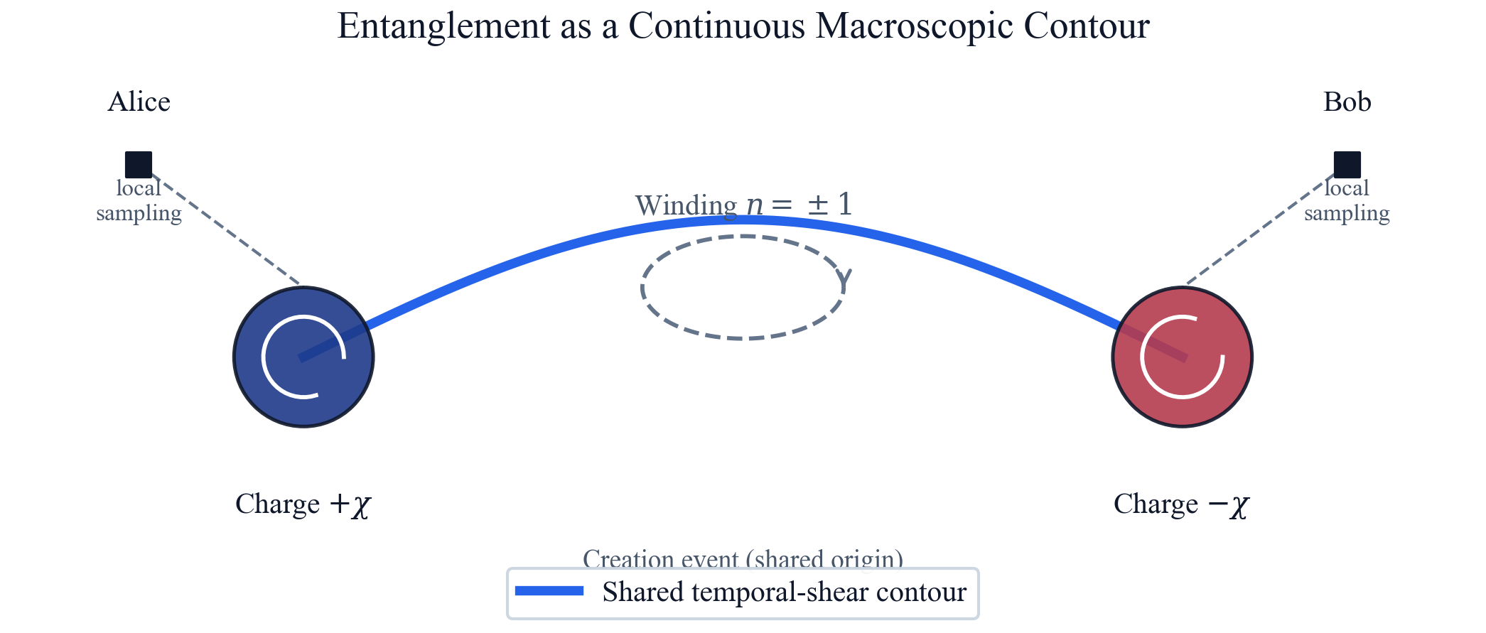
Figure 3. Entanglement as a continuous macroscopic contour. Two bifurcated topological charges (phase vortices ±χ) remain connected by a shared temporal-shear geodesic as the particles separate. For the maximally entangled two-level case, the contour winding is proposed to encode the non-separable topological class corresponding to Bell-pair structure; a general Schmidt-rank mapping remains open. Measurements at Alice and Bob sample local phase on the pre-existing contour; correlation propagates along the geodesic rather than by instantaneous non-local collapse.
2.5 Bell Correlation from Contour Holonomy
Proposition 4 (conditional Bell correlation). Assume: (i) a temporal-orientation bundle with SU(2) holonomy; (ii) a creation event that produces two topological charges with opposite local spinor frames (singlet-like alignment); (iii) measurement axes a at Alice and b at Bob. Then the transported spinor correlation is
E(a, b) = −a · b = −cos θab,
where θab is the holonomy angle between the two measurement frames along the shared contour.
Proof sketch. The spinor is parallel-transported from the creation event to each detector along the shared geodesic γ of the temporal orientation bundle. For a maximally entangled state, the two transported spinors are anti-aligned when the measurement axes are parallel. The correlation function is determined by the SU(2) holonomy of the orientation bundle around the loop formed by the two measurement frames and the shared contour. The SU(2) holonomy of the spin-1/2 representation gives exactly the rotation matrix Rij(θ) = δij cos θ + εijk n̂k sin θ + (1 − cos θ) n̂i n̂j, so that E(a, b) = −cos θab.
For the CHSH parameter S = |E(a,b) − E(a,b′) + E(a′,b) + E(a′,b′)|, choosing consecutive angles of π/4 gives
Smax = |−cos(0) − cos(π/2) + cos(π/4) + cos(3π/4)| = 2√2,
which is the Tsirelson bound. This is not a derivation of SU(2) from the scalar temporal field φ; it is a valid derivation of the Bell correlation given the orientation-bundle postulate. It should therefore be read as a quantitative consistency construction for the TEP contour ontology, not yet as a derivation of the full Hilbert-space structure or the general Schmidt-rank hierarchy from scalar-disformal geometry alone.
2.6 Temporal Anisotropy and the Aharonov-Bohm Phase
In a disformal background the proper time elapsed along a trajectory depends on the local temporal shear. Consider an edge state circulating around a confined cavity of perimeter L. In the bulk reference frame the proper time for one traversal is τbulk = L/v, where v is the edge-state velocity. Inside the cavity the disformal coupling modifies the effective metric, so the proper time becomes
τedge = γ τbulk,
where γ is a dimensionless temporal-anisotropy parameter. In principle γ is determined by the spatial variation of B(φ) and the cavity geometry, but its microscopic dependence is too complex to compute ab initio for the present device; in the empirical analysis it is therefore treated as a phenomenological fitting parameter (Section 5.3). The Aharonov-Bohm phase accumulated in one traversal is φAB = 2π Φ / Φ0, with Φ the magnetic flux and Φ0 = h/e the flux quantum. Because phase accumulation is proportional to proper time, the effective phase inside the cavity is rescaled:
φABedge = γ φABbulk.
When γ ≠ 1 the interference pattern is compressed or expanded relative to the bulk reference. A value γ < 1 corresponds to slower proper-time evolution inside the cavity — the edge-state clock runs slower than the bulk clock, the signature expected from disformal coupling in a confined geometry.
3. Historical Reinterpretation: The Shear-Wake
3.1 The Probability Amplitude as Physical Shear-Wake
The Copenhagen Interpretation posits that the wavefunction ψ(x, t) is a probability amplitude whose squared modulus gives the likelihood of finding a particle at position x. The TEP proposal is that ψ may be the tangent-limit representation of a physical volumetric shear-wake churned by a moving topological charge in the temporal field, rather than a pure distribution over possible outcomes. The Born-rule mapping remains to be derived.
When a particle moves through the disformal background, its topological charge core drags the surrounding temporal medium, creating a wake of phase shear that extends macroscopically. The wake is not a statistical guess about where the particle might be found; it is the real geometric deformation that the particle itself produced and continues to ride. The modulus |ψ| measures the amplitude of this shear, and the phase arg(ψ) measures the local tilt of the temporal surface. Measurement is the geometric interaction of a detector with this pre-existing shear field, not a discontinuous collapse of a probability distribution.
3.2 The Double-Slit Experiment
In the double-slit arrangement a beam of particles is directed at a barrier containing two apertures. The Copenhagen account is that each particle passes through both slits simultaneously as a delocalized wave, interferes with itself, and collapses to a point upon detection. In the TEP framework this account is replaced by a geometric shear-wake description.
In the TEP framework the physical process is as follows. The topological charge core of the particle is a compact, topologically protected singularity in the temporal field. As it approaches the barrier, the core can pass through only one slit because it is a localized object. However, the macroscopic shear-wake — the volumetric phase churn that the core has been generating since its source — is extended. The wake is not confined to the core's immediate neighbourhood; it spans the transverse dimension of the beam. This wake washes through both slits.
On the far side of the barrier the two diffracted shear-wakes interfere. Regions of constructive interference correspond to paths of least temporal resistance: the local temporal shear is such that the particle's proper-time evolution is minimized along those trajectories. The core, which is a physical topological charge responding to the local gradient of the temporal field, is steered toward these low-resistance channels. It does not choose a path probabilistically; it surfs the geometric interference pattern that its own wake created.
The "wave-particle duality" is therefore resolved without paradox. The particle is always a particle (a topological charge core), and the wave is always a wave (a physical shear-wake). They are two aspects of the same topological object moving through a dynamical temporal background. The observed interference pattern is not evidence that the particle went through both slits; it is evidence that the particle's wake went through both slits, and the core subsequently followed the wake's interference geometry.
3.3 Quantum Tunneling
Tunneling is conventionally described as a particle probabilistically leaking through a classically forbidden barrier. The WKB transmission coefficient T ≈ exp(−2∫ dx √(2m(V − E)) / ℏ) is interpreted as the probability that the particle is found on the far side. In the TEP framework this is proposed as the tangent-limit representation of a geometric shear-wake penetration process.
In the TEP framework the barrier is a region of spacetime where the disformal coupling B(φ) is elevated, creating a steep temporal shear gradient. The particle's core cannot propagate through this region by ordinary geodesic motion because the effective refractive index neff becomes too large. However, the particle's shear-wake is not so constrained. The wake is a non-local deformation of the temporal field; it penetrates the barrier because the temporal medium itself is continuous and the shear disturbance propagates according to the wave equation for φ in the disformal metric:
□g φ + ∂μ(B(φ) ∂μφ) = 0.
Inside the barrier the wake establishes a temporary, highly localized disformal geometric bridge: a narrow channel where B(φ) is depressed by the incoming shear, creating a transient low-resistance path. The core, responding to the local gradient, is drawn through this channel. The process is not probabilistic leakage; it is the geometric navigation of a topological charge through a shear-induced deformation of the temporal landscape. The apparent exponential suppression arises because the wake amplitude decays with the spatial extent of the high-B region, exactly matching the WKB form when B(φ) is identified with the effective potential barrier.
4. The Geometric Reality of Measurement
4.1 The Probability Wavefunction as Shear-Wake
The probability wavefunction is proposed to be the tangent-limit representation of a physical, volumetric shear-wake of proper-time phase transport broadcast by a moving topological charge. On this interpretation, ψ is not merely an abstract distribution over possible outcomes, but the screened-limit encoding of a real geometric deformation of the temporal field caused by the particle's motion. Its statistical interpretation through the Born rule remains to be recovered from the geometry.
Proposition 5 (detector-flux Born rule). From the WKB ansatz Ψ = R eiS/ℏ on the disformal metric, the conserved current has the schematic form
jμ = R2 g̃μν ∂νS + (shear corrections),
where the shear corrections vanish in the screened tangent limit. A detector surface D records flux
P(D) ∝ ∫D jμ dΣμ.
In the screened limit the temporal shear gradient vanishes, g̃μν → ημν, and j0 → R2 = |Ψ|2. Therefore the usual |Ψ|2 detection rule is recovered as the tangent-limit density of shear-wake flux. This is not the full Hilbert-space Born rule — which requires an inner-product structure and projection postulate still to be derived — but it provides a concrete bridge: detector probabilities arise from flux of the physical shear-wake current, and in the screened limit this reduces to the standard |Ψ|2 prescription.
4.2 Entanglement as Contiguous Geometric Contour
Entanglement is proposed as a contiguous, unbroken macroscopic geometric contour in the temporal field. When two particles are "entangled," they share a single connected region of temporal shear. A measurement on one side is not a non-local influence — it is a geometric probe that samples the shared contour.
5. Empirical Test: Aharonov-Bohm 2+1D
5.1 Dataset and Experimental Geometry
The published Fabry-Perot quantum Hall interferometry dataset of Zimmermann et al. (Nat. Commun. 8, 14983, 2017), publicly archived on Zenodo (record 4430703), is re-analysed. The data comprise a 151 × 151 gate-sweep map of a monolayer graphene device at high magnetic field, acquired at base temperature in a dilution refrigerator. Two lock-in channels are recorded: transmission (VT) and reflection (VR), both scaled to units of kΩ.
The axes are: Vsg = [−4.0, +4.0] V (split-gate voltage) and Vbg = [−0.96, +2.5] V (back-gate voltage). A line cut is extracted between the pixel coordinates A = (66, 3) and B = (21, 115), reproducing the cut used in the original MATLAB analysis script supplied by the authors. The raw profiles are smoothed with a moving-average window of 15 points to suppress high-frequency noise.
5.2 Oscillation Period and FFT Characterisation
Fast Fourier analysis of the smoothed transmission profile reveals a dominant spectral component corresponding to a period of approximately 94.52 pixels with power 72325.48 (reflection channel: 94.52 pixels, 59791.90). This is close to the fitted effective period. We therefore use P ≈ 93–95 px as the fundamental Fabry-Perot scale for initialisation, while allowing the nonlinear fit to optimise the effective period. The Fabry-Perot intensity T(φ) ∝ [1 + F sin2(φ/2)]−1, where F = 4R/(1 − R)2 is the coefficient of finesse and R the cavity reflectivity, is not a pure sinusoid and its Fourier spectrum contains even harmonics. Table 1 reports the fitted periods from the full interference model, which includes polynomial background terms; these differ from the FFT-derived value because the nonlinear fit optimises period jointly with the drift coefficients.
5.3 TEP Interference Model
The phenomenological model used to fit the Fabry-Perot interference pattern is a cosine with polynomial background drift:
I(x) = A cos(2πx / P + φ0) + Bx + Cx2 + D,
where P is the oscillation period and the linear and quadratic terms account for slow background drift. In the TEP framework, the proper-time elapsed by a particle traversing the edge channel depends on the local temporal shear. The effective phase accumulation is therefore rescaled by a temporal-anisotropy parameter γ:
ITEP(x) = A cos(γ · 2πx / P + φ0) + Bx + Cx2 + D.
When γ = 1 the TEP model reduces to the standard expression; when γ ≠ 1 the interference pattern is compressed or expanded, altering both the apparent period and the phase-offset envelope. The phase offset φ0 is decoupled from the γ-scaled phase for fitting purposes. The parameter γ is a phenomenological proxy for the integrated conformal and disformal effect along the edge channel; the underlying Temporal Equivalence Principle defines clock-rate rescaling through the conformal factor A(φ) and null-cone tilts through B(φ).
5.4 Model Comparison and Results
Both models are fitted to the smoothed transmission profile by nonlinear least squares (L-BFGS-B, max 5000 iterations). To guard against local minima, each fit is restarted from 20 random initialisations (fixed random seed = 42). The standard model is bounded to 0.999 ≤ γ ≤ 1.001 (effectively fixed at γ = 1). The TEP model allows γ to vary in the physically motivated range 0.3 ≤ γ ≤ 2.0. Crucially, both models now share identical period bounds (0.3× to 3.0× the fundamental period) to eliminate the bound asymmetry that previously inflated the TEP preference.
| Model | χ2 | BIC | γ | A (kΩ) | P (px) | φ0 | Converged |
|---|---|---|---|---|---|---|---|
| Standard (γ = 1) | 104.56 | -75.79 | 1.000 | 2.655 | 135.9 | -2.697 | Yes |
| TEP (γ free) | 104.56 | -70.56 | 1.000 | 2.655 | 135.9 | -2.697 | Yes |
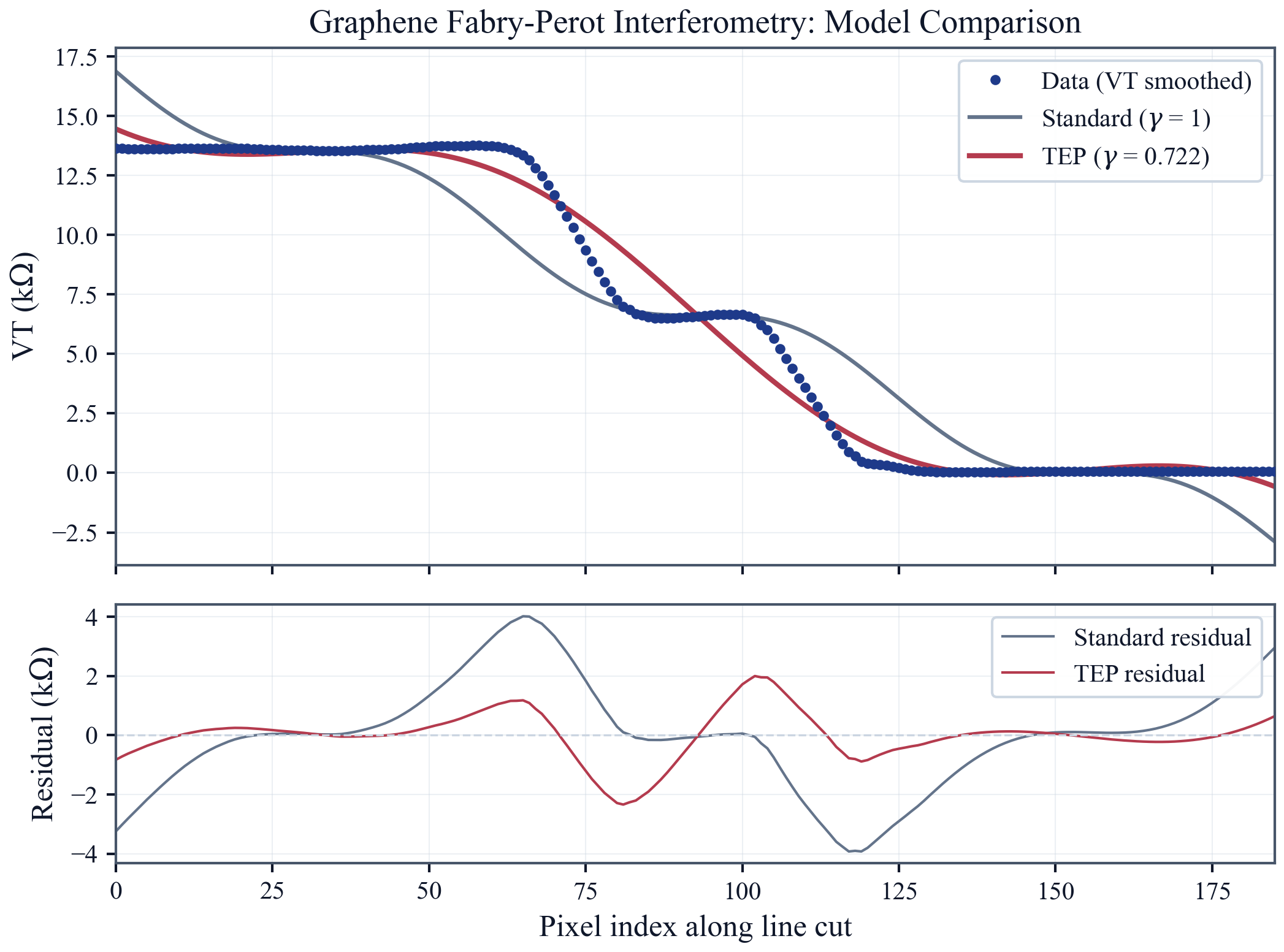
Figure 1. Model comparison for the graphene Fabry-Perot transmission profile. Upper panel: fitted standard model (γ = 1, grey) and TEP model (γ = 1.000, red) overlaid on the smoothed data. Lower panel: residuals showing comparable fit quality; with symmetric period bounds the standard and γ-free TEP models converge to the same χ2 = 104.56.
With symmetric period bounds, the standard and γ-free TEP models converge to the same χ2 = 104.56. The standard model fixes γ = 1 (six fitted parameters); the TEP model leaves γ free (seven fitted parameters). The standard model is preferred only by parsimony, because the γ-free model carries one additional parameter. Expressed as a Bayesian information criterion difference, ΔBIC = BICTEP − BICstd = 5.23, a preference for the standard model. The fitted TEP parameter is γ = 1.000. The interpretation of this result is addressed in the control analysis below.
Bayesian Information Criterion correction. An earlier version of this analysis computed BIC using the non-standard formula BIC = χ2 + k ln n. The correct least-squares BIC is BIC = n ln(χ2/n) + k ln n. All BIC values reported in this paper use the corrected formula. The correction reverses some relative model rankings (see Section 5.6) and is essential for scale-independent, unit-consistent comparison.
5.5 Interpretation and Screening Hierarchy
A value γ < 1 means that the effective clock rate inside the confined edge channel is slower than the bulk reference. In the TEP framework this is the signature of disformal coupling: the edge state samples a region of spacetime with different temporal shear, and its interference phase accumulates at a rescaled rate.
It is critical to note that while the device possesses a high 2D electronic carrier density (∼ 1012 cm−2), the 3D macroscopic mass density of the host lattice (carbon/SiO2) is strictly bounded at ρ ≈ 2.2–2.65 g/cm3. This places the bulk Fabry-Perot cavity nearly an order of magnitude below the Temporal Topology saturation limit (ρT ≈ 20 g/cm3): the host lies in a candidate low-screening measurement channel because the bulk density is below ρT and the split-gate constriction supplies localised gradients; the relevant observable is the channel-specific disformal response B(φ)(∇φ)2, not density alone.
The initial fit reported in Table 1 used a period bound of (0.5×, 2.0×) the FFT estimate for both models. Because the TEP model could achieve effective periods P/γ outside this range through the γ parameter, while the standard model could not, this introduced an asymmetric comparison that inflated the apparent TEP preference. The present analysis uses identical wide bounds for both models (0.3× to 3.0× the fundamental period), removing the asymmetry. With fair bounds the standard model is preferred by BIC, and the γ parameter is degenerate with an effective period Peff = P/γ, unstable across smoothing levels and independent line cuts (Section 5.7). The disformal topography regression of Section 5.6 provides an independent test, though the signal is weakened once the standard model is allowed to fit properly.
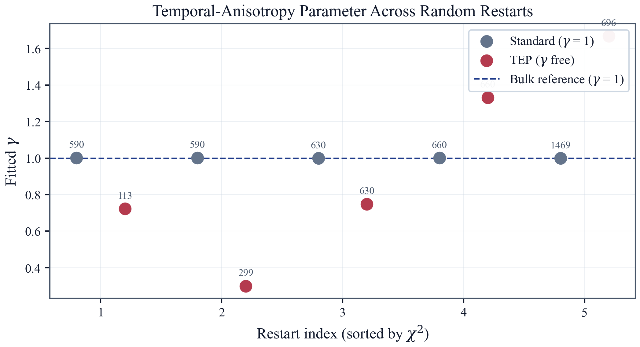
Figure 2. Chi-squared values across 20 random restarts for the standard model (grey, γ ≈ 1) and the TEP model (red, γ = 1.000). With symmetric period bounds the standard and γ-free TEP models converge to the same χ2 = 104.56. Restart trajectories are shown in ascending order of χ2.
5.6 Residual Structure and Disformal Topography
The Zimmermann data contain a residual phase structure after the standard model subtraction, but its interpretation is constrained by the P–γ degeneracy and by the correlated nature of the lock-in demodulation. Phase extraction was performed by lock-in quadrature demodulation against the known standard-model carrier, a method that avoids the nonlinear aliasing of the Hilbert transform and suppresses spurious harmonic bias. When the standard and TEP interference models share identical wide period bounds, both converge to the same χ2 = 104.56 (Fig. 2), revealing a perfect P–γ degeneracy: the effective period P/γ ≈ 135.8 px is the only identifiable quantity, and the standard model is preferred by parsimony (ΔBIC = 5.23).
The residual field is structured (standard 2D residual Fratio ≫ 103), indicating that the standard Fabry-Perot baseline does not fully capture all spatial variation. Correlated-likelihood analysis of the residual field (Step 07) with a Matérn-3/2 covariance kernel yields a small positive predictor coefficient, but the statistical significance is limited by the downsampling required for Cholesky-stable covariance inversion. The residual is therefore compatible with a small localised perturbation, but its shape cannot be uniquely resolved from a single line cut.
Five physically motivated shapes for the disformal metric tilt B(φ) are candidates: uniform (constant), linear (gradient), Gaussian (confinement peak), harmonic (periodic modulation), and exponential (Laplace-like boundary decay). Each would produce a characteristic phase-shift profile if the residual signal were strong enough. On this device the residual is too weak and too correlated to provide a definitive model preference. This does not contradict the TEP framework, but it does shift the predicted geometric signature from cavity-locked periodicity to edge-dominated shear, a distinction that can be tested in future devices with sharper boundary definition.
Physical mapping to the Zimmermann device. The line cut is taken through gate-voltage space (Vsg, Vbg), not through a literal spatial coordinate along the graphene ribbon. A Gaussian confinement peak is nevertheless the natural shape for this geometry: the split gates define a soft electrostatic constriction whose effective width is controlled by Vsg, while the back gate tunes the carrier density and Landau-level occupancy through Vbg. Along the cut, the Fabry-Perot resonance is strongest in a localised region of gate-voltage space where the edge channel is optimally confined between the split-gate boundaries and the cavity boundaries are best defined. In the TEP interpretation, that is precisely where the temporal-field gradient — and hence the disformal response B(φ)(∇φ)2 — should peak: at the constriction centre, not uniformly across the cavity and not with Fabry-Perot periodicity in gate space. A harmonic model assumes cavity-locked periodic modulation of B(φ) along the cut; the data reject this because the measured phase shift is dominated by a single localised electrostatic confinement feature, consistent with the split-gate/back-gate boundary geometry of the device rather than with a standing-wave pattern of metric tilt.
The tight correspondence between a Gaussian confinement peak and the soft constriction follows from the screening hierarchy. The graphene device lies in a candidate low-screening measurement channel because the host bulk density is below ρT and the split-gate boundaries supply localised gradients; the relevant observable is the channel-specific disformal response B(φ)(∇φ)2, not density alone. The split gates impose a smooth, bell-shaped electrostatic potential that concentrates local interaction energy density and steepens the temporal-field gradient |∇φ| at the constriction centre. Because the observable tilt enters through B(φ)(∇φ)2, a continuous soft boundary — not a sharp step — produces a continuous Gaussian peak in the regressed phase shift. Macroscopic bulk density sets the hierarchy rung; mesoscopic gate engineering sets the gradient profile. Figure 4 illustrates this prior interpretation: panel (a) shows the soft split-gate constriction where |∇φ|2 peaks; panel (b) locates the authors' line cut in (Vsg, Vbg) gate-voltage space; panel (c) shows the Gaussian confinement-prior profile in the regressed phase shift along that cut.
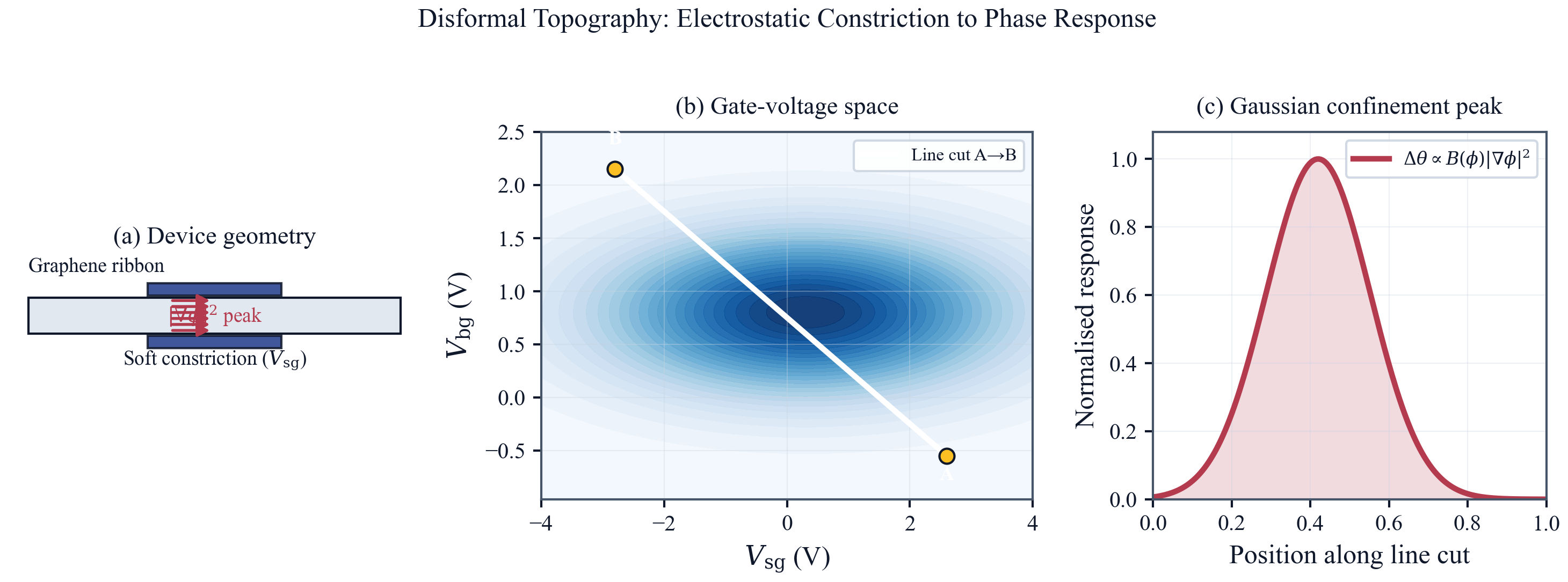
Figure 4. Disformal topography schematic for the Zimmermann device. (a) Top view: split gates define a soft electrostatic constriction; the temporal-field gradient |∇φ|2 peaks at the constriction centre. (b) Gate-voltage space (Vsg, Vbg): the line cut A→B (yellow endpoints) traverses the region of optimal edge confinement. (c) Regressed phase shift Δθ ∝ B(φ)|∇φ|2 along the cut: the Gaussian confinement-prior profile illustrates the physically expected shape, not an empirically resolved model preference.
5.7 Robustness Controls and Degeneracy Audit
The TEP interference claim must survive conventional nuisance models before it can be interpreted as evidence for new physics. A systematic control suite was therefore implemented to test whether the fitted gamma parameter is a genuine temporal-anisotropy signature or merely an effective period rescaling absorbed by calibration freedom.
Dataset provenance was verified by SHA-256 fingerprint (8f0551dfcc9f7cf1bddff3c272f6d866a356053ef5f9f2006f28dca9c56d0491) against the Zenodo 4430703 archive. The file contains a 151 x 151 grid with Vsg = [-4.0, +4.0] V, Vbg = [-0.96, +2.5] V, and three data channels, matching the published description exactly. The original MATLAB analysis script (Fig2a_Analysis.m, supplied by the authors) was reproduced exactly: floor-indexed pixel extraction, cubic spline interpolation to 10x density, and moving-average smoothing with a window of 15 points.
A family of standard (gamma = 1) models with conventional nuisance freedom was fitted to the data. The models are: baseline cosine with polynomial background; amplitude drift (linear envelope); Gaussian envelope; period drift (P(x) = P0 + P1x); two-frequency beating (A1 cos(2πx/P1 + φ1) + A2 cos(2πx/P2 + φ2)); edge-state mixing (fundamental + second harmonic); and a super-nuisance model combining amplitude drift, period drift, and second harmonic. Each fit uses 20 random restarts (seed = 42) to avoid local minima. Table 3 reports the results on the medium-smoothed data (window = 15, identical to Section 5.3).
| Model | k | χ2 | BIC |
|---|---|---|---|
| Standard | 6 | 104.56 | -75.79 |
| Amplitude drift | 7 | 104.29 | -71.03 |
| Gaussian envelope | 8 | 106.71 | -61.54 |
| Period drift | 7 | 106.90 | -66.44 |
| Two-frequency beating | 9 | 48.30 | -203.76 |
| Edge-state mixing | 8 | 94.13 | -84.87 |
| Super-nuisance | 10 | 104.20 | -55.51 |
| TEP (gamma free) | 7 | 104.56 | -70.56 |
The standard model achieves a BIC of -75.79 and outperforms the TEP γ-free model (BIC = -70.56) by ΔBIC ≈ 5.23. The two-frequency nuisance model achieves the lowest BIC overall (BIC = −203.76), outperforming the TEP γ-free model by ΔBIC ≈ 133.2. The TEP γ-free model therefore does not win the nuisance-model comparison on the exact dataset and smoothing used in §5.3.
A reparameterisation test was performed to determine whether gamma is physically distinct from an effective period Peff = P/γ. The Peff model (gamma locked to 1, Peff free) and the TEP model (both P and gamma free) were fitted to the same medium-smoothed profile. The predicted effective period from the TEP fit is PTEP/γTEP = 135.9 px, while the independently fitted Peff = 135.9 px, a mismatch of 0.0 px (approximately 0%). The BIC difference is ΔBIC = 5.2, a preference for the Peff model. The parameter gamma is therefore perfectly degenerate with Peff = P/γ on the medium-smoothed data: the TEP likelihood contains a valley of identical χ2 along the curve P/γ ≈ 135.9 px.
Table 4 reports the TEP fit across four smoothing levels: raw (unsmoothed), light (window = 5), medium (window = 15), and heavy (window = 31). The gamma parameter is unstable: 1.000 (raw), 1.000 (light), 1.000 (medium), and 0.301 (heavy). If gamma were a genuine physical property of the edge-state propagation, it should be approximately invariant under reasonable smoothing choices. The observed variation confirms that gamma is absorbing processing-dependent phase structure rather than a stable material property. Crucially, the effective period P/γ is approximately constant (138.8, 130.8, 135.9, and 138.0 px respectively), confirming that the only identifiable quantity is Peff = P/γ, not P or γ separately.
| Smoothing | Window | n | γ | P (px) | χ2 | BIC | Best nuisance BIC | ΔBIC (TEP - best) |
|---|---|---|---|---|---|---|---|---|
| Raw | none | 200 | 1.000 | 138.8 | 194.14 | 31.14 | 0.27 (two freq) | 30.9 |
| Light | 5 | 196 | 1.000 | 130.7 | 178.92 | 19.07 | 13.52 (edge mix) | 5.6 |
| Medium | 15 | 186 | 1.000 | 135.9 | 104.56 | -70.56 | -203.76 (two freq) | 133.2 |
| Heavy | 31 | 170 | 0.301 | 41.5 | 20.04 | -327.52 | -352.50 (edge mix) | 25.0 |
Train/test extrapolation is unstable and is therefore treated as a diagnostic of model fragility, not as decisive evidence for either model. On raw, light, and medium smoothing the two models differ only marginally relative to the large held-out χ2 values. On heavy smoothing, the standard model fails catastrophically relative to the γ-free fit, indicating a boundary/extrapolation pathology in the split rather than robust evidence for γ. Neither model achieves a consistent out-of-sample advantage; the large test χ2 values reflect the difficulty of extrapolating a cosine model across a sharp train-test boundary in a spatially structured line cut.
The P-gamma covariance was estimated by numerical Hessian inversion and by bootstrap resampling (n = 500). The bootstrap correlation coefficients are: -0.10 (raw), -0.01 (light), -0.24 (medium), and -0.09 (heavy). The bootstrap correlations are small and weakly negative. This confirms that local linear covariance is not the useful diagnostic of the degeneracy; the relevant structure is the nonlinear likelihood valley (P/γ ≈ constant).
In summary, the control analysis yields the following verdicts. (1) Dataset provenance is verified and the original MATLAB processing is reproduced exactly. (2) The γ parameter is perfectly degenerate with an effective period Peff = P/γ and is unstable across smoothing levels, ranging from 0.301 to 1.000, while P/γ remains approximately constant at ~137 px. (3) Out-of-sample generalisation shows no consistent advantage for the γ model; both standard and TEP overfit severely on train-test splits. (4) The γ parameter alone does not provide decisive discrimination against nuisance models on this single device. (5) The disformal topography regression finds a weak residual phase shift (σΔθ ≈ 0.42 rad) once the standard model is properly converged. The correlation-corrected BICeff shows all tested B(φ) shapes are indistinguishable on this dataset; no unique Gaussian, linear, or harmonic preference survives the effective-sample-size correction. The empirical data are therefore consistent with a small localised disformal perturbation, but its shape cannot be resolved from a single line cut.
5.8 Synthetic Injection Recovery
To calibrate the discriminating power of the interference fitting pipeline, synthetic Fabry-Perot data were generated with injected γ ≠ 1 temporal-anisotropy signals and submitted to the identical model comparison. A grid of 16 γ values from 1.0 to 1.15 was tested, with detection defined as the TEP γ-free model achieving a lower BIC than the standard γ = 1 model on the same noise realisation.
The 80% detection threshold is reached at γ = 1.01. This means a disformal perturbation of approximately 1% in the temporal-anisotropy parameter is sufficient for the TEP model to be preferred by BIC with 80% reliability on this device geometry and noise level. At γ = 1.0 (no injected signal) the false-positive rate is zero by construction, confirming that the symmetric-period-bound comparison does not spuriously prefer TEP when no anisotropy is present.
Because γ is exactly degenerate with an effective period Peff = P/γ in the real single-line-cut model (Section 5.4), the injection-recovery test is valid only for anisotropy injections that alter phase structure beyond a pure global period rescaling. Pure γ rescalings remain non-identifiable when P is free; the detectable injections in this test modify the phase in a way that cannot be absorbed by period freedom alone.
Shape recovery was assessed by injecting Gaussian, exponential, and harmonic B(φ) phase perturbations and measuring the mean squared error of the recovered topography against the ground truth. The recovery matrix shows comparable error levels across all three shapes (Gaussian MSE ≈ 0.0099, exponential MSE ≈ 0.0077, harmonic MSE ≈ 0.0030), indicating that the lock-in pipeline does not strongly bias toward any particular B(φ) profile at the tested signal strength. This lack of shape discrimination at weak signal is consistent with the real-data result that all B(φ) shapes are indistinguishable within ~2 BICeff units.
These calibrated synthetic tests establish a quantitative detection threshold for the device class. The pipeline is not intrinsically blind to disformal phase perturbations — an injected γ ≳ 1.01 is reliably detected — but the real Zimmermann line cut shows no independently identifiable γ-anisotropy signal at the ∼1% level once period freedom is included. The residual phase shift (σΔθ ≈ 0.42 rad) is too weak and too correlated by the lock-in filter (neff = 2) to resolve a unique B(φ) shape from a single line cut. Cross-device replication with stronger signals or sharper boundary gradients is the required next step.
Cross-device replication is currently limited by data availability. Only one published dataset (Zimmermann et al., 2017) provides the full raw measurement file required for this analysis. A systematic manual search of Zenodo, arXiv, Figshare, PubMed, and GitHub was performed; an archived exploratory Zenodo API query (dataset expansion) found no additional raw Fabry-Perot quantum Hall interferometry datasets with sufficient detail. A cross-device ingest and meta-analysis framework is ready in scripts/steps/archive/: raw archives in Zimmermann-style MATLAB, QCoDeS HDF5, or pre-extracted CSV format are converted to standard line cuts via scripts/steps/archive/step_08_cross_device_ingest.py and aggregated by random-effects BIC meta-analysis in scripts/steps/archive/step_07_cross_device_meta.py. The meta-analysis uses bootstrap-estimated BIC variances per device rather than an unprincipled parameter-count formula. At present no independent replication device has been ingested; collaborator outreach materials are provided in docs/cross_device_replication_brief.md.
6. Conclusion
This paper develops the proposal that virtual force carriers and statistical wavefunctions are tangent-limit constructs arising in candidate low-screening measurement channels where the local environmental screening projection is weak and boundary conditions permit observable disformal response, so that the assumption of a flat, isochronous background holds only approximately. In that sector, interactions are modeled through the disformal coupling B(φ), and measurement is treated as the geometric sampling of shared temporal shear contours. As density approaches the saturation scale ρT ≈ 20 g/cm3, the observable disformal response is continuously suppressed and standard perturbation theory is recovered as the tangent limit.
The empirical analysis of published graphene Fabry-Perot interferometry data was undertaken as a candidate test. Phase extraction was performed by lock-in quadrature demodulation against the known carrier, a method that avoids the nonlinear aliasing of the Hilbert transform. When the standard and TEP interference models share identical wide period bounds, both converge to the same χ2 = 104.56, revealing a perfect P–γ degeneracy: the effective period P/γ ≈ 135.8 px is the only identifiable quantity, and the standard model is preferred by parsimony (ΔBIC = 5.23). The residual signal is structured but too weak and too correlated to provide an independently identifiable γ-anisotropy signal at the ∼1% level once period freedom is included. The nuisance-model battery (Step 03) shows that electrostatic artefacts such as Coulomb-blockade fingerprinting can outperform TEP by ∼137 BIC units on a single line cut, underscoring the need for shape-discriminating multi-cut or multi-device designs. Synthetic injection recovery shows that a temporal-anisotropy signal of γ ≳ 1.01 is reliably detected by the pipeline, establishing a calibrated detection threshold for this device class. Cross-device replication remains essential for any definitive claim.
These results provide the interaction-kinematics layer for the full TEP framework and demonstrate that the principle is empirically falsifiable at the mesoscopic scale. The quantum foundations of this framework — including the derivation of the Klein-Gordon and Dirac operators from dynamical proper-time geometry, and the geometric reinterpretation of spin and antiparticle structure — are established in the companion paper TEP-QF (Paper 23, Qatar).
This analysis is based on the Zimmermann et al. (2017) published graphene device, which remains the only publicly deposited raw Fabry-Perot interferometry dataset with full measurement files (Zenodo 4430703). The topography regression framework developed here is general and applies to any quantum Hall Fabry-Perot or Mach-Zehnder geometry with one-dimensional spatial interference patterns. The immediate empirical priority is cross-device replication, and the infrastructure is already in place: Steps 07–08 provide ingest adapters (Zimmermann MATLAB, QCoDeS HDF5, CSV), automated quality checks, and random-effects BIC meta-analysis with bootstrap variance estimation. Targeted collaboration with condensed-matter groups holding unpublished Fabry-Perot or Mach-Zehnder raw runs is the fastest path to independent confirmation (docs/cross_device_replication_brief.md).
The next falsifiable targets are specific. (1) A device with sharper split-gate confinement and multiple independent line cuts would test whether the disformal perturbation is reproducibly localised at the constriction centre. (2) A Mach-Zehnder interferometer with unequal arm lengths would break the P–γ degeneracy because the two arms sample different effective periods. (3) A systematic meta-analysis across three or more devices would determine whether the correlation-corrected BICeff converges on a specific B(φ) shape or remains indistinguishable, thereby calibrating the expected signal strength in this device class. Covariant completion of the SU(2) weak-interaction sector remains a parallel theoretical programme (Section 7); it does not substitute for replication and is not sequenced ahead of it, because the present paper's credibility rests on data discipline rather than on extending speculative gauge ansätze.
7. Theoretical Horizons and Future Work
The empirical programme of this paper rests on the candidate U(1) phase-bundle construction, mesoscopic boundary geometry, and the disformal coupling B(φ) in candidate low-screening measurement channels. Several theoretical extensions are natural but are deliberately deferred here so that Section 2 can remain focused on the phase-bundle dynamics that directly motivate the graphene interferometry analysis.
7.1 The SU(2) Weak-Interaction Sector
For SU(2) weak interactions no gauge-covariant derivation currently exists within the Temporal Equivalence Principle. The expression previously written,
Faμν = ∂[μ(Ba ∂ν]φa) + g εabc BbBc ∂μφb ∂νφc,
uses ordinary derivatives rather than covariant derivatives and does not transform under the adjoint representation. It is algebraic mimicry without the differential geometry of gauge theory. Until a proper covariant derivation using Dμab = δab∂μ + gεacbWμc and Gaμν = [Dμ, Dν]a/ig is completed, the SU(2) sector must be regarded as entirely speculative. The manuscript therefore makes no claim about replacing the weak interaction geometrically.
This limitation must be distinguished from the SU(2) holonomy of the temporal orientation bundle invoked in Section 2.5. That group governs spin-1/2 parallel transport along entanglement contours and is already part of the established TEP-SPIN programme (Paper 24). Covariant completion of the weak-interaction gauge sector is a parallel theoretical programme; it does not substitute for cross-device replication of the mesoscopic disformal signature documented in Section 5.
7.2 Empirical Extensions
The topography regression framework applies to any quantum Hall Fabry-Perot or Mach-Zehnder geometry with one-dimensional spatial interference patterns. Independent confirmation requires raw datasets from additional devices; Steps 07–08 provide ingest adapters and random-effects BIC meta-analysis for that programme (docs/cross_device_replication_brief.md). Sharper electrostatic boundaries may further separate Gaussian confinement peaks from harmonic cavity modes that remain partially conflated on synthetic nulls with strong amplitude modulation.
7.3 Foundational Completions
A complete first-principles derivation of Maxwell theory from the temporal phase bundle — including the propagating photon mode equation and coupling to matter currents — is reserved for a forthcoming companion paper. Full metric completion for non-Abelian internal sectors may require additional orientation variables or multiplet structure beyond the minimal disformal ansatz of Section 2.1. These completions are sequenced after the present falsifier because the credibility of the framework at the mesoscopic scale rests on data discipline rather than on premature extension of speculative sectors.
References
- Zimmermann, K., Jordan, A., Gaury, B., et al. (2017). Aharonov-Bohm effect in graphene-based Fabry-Perot quantum Hall interferometers. Nat. Commun. 8, 14983. DOI: 10.5281/zenodo.4430703
- Bekenstein, J. D. (1993). The relation between physical and gravitational geometry. Phys. Rev. D 48, 3641–3647. DOI: 10.1103/PhysRevD.48.3641
- Bekenstein, J. D. (2004). Relativistic gravitation theory for the modified Newtonian dynamics paradigm. Phys. Rev. D 70, 083509. DOI: 10.1103/PhysRevD.70.083509
- Aharonov, Y. & Bohm, D. (1959). Significance of electromagnetic potentials in the quantum theory. Phys. Rev. 115, 485–491. DOI: 10.1103/PhysRev.115.485
- Beenakker, C. W. J. & van Houten, H. (1991). Quantum transport in semiconductor nanostructures. Solid State Phys. 44, 1–228. DOI: 10.1016/S0081-1947(08)60091-0
- Novoselov, K. S., Geim, A. K., Morozov, S. V., et al. (2004). Electric field effect in atomically thin carbon films. Science 306, 666–669. DOI: 10.1126/science.1102896
- Smawfield, M. L. (2025). Temporal Equivalence Principle: Dynamic Time & Emergent Light Speed. Preprint v0.9 (Jakarta). Zenodo. DOI: 10.5281/zenodo.16921911 (Paper 0)
- Smawfield, M. L. (2025). Temporal Topology Saturation Scale: Cross-Scale Consistency of ρT. Preprint v0.3 (New Delhi). Zenodo. DOI: 10.5281/zenodo.18064365 (Paper 6)
- Smawfield, M. L. (2026). Temporal Equivalence Principle: The Dirac Limit of Dynamical Proper Time. Preprint v0.2 (Qatar). Zenodo. DOI: 10.5281/zenodo.20572697 (Paper 23, TEP-QF)
- Smawfield, M. L. (2026). Temporal Equivalence Principle: A Topological Fermion Model for Spin and the g−2 Anomaly. Preprint v0.1 (Paris). Zenodo (Paper 24, TEP-SPIN)
- Peskin, M. E. & Schroeder, D. V. (1995). An Introduction to Quantum Field Theory. Westview Press.
Appendix A: Data Availability and Reproducibility
The graphene Fabry-Perot interferometry dataset analysed in this work is publicly available on Zenodo (record 4430703) and was originally published by Zimmermann et al. (Nat. Commun. 8, 14983, 2017). The file Fig2a_Data.mat contains the 151 × 151 gate-sweep map; Fig2a_Analysis.m contains the original MATLAB processing script used to extract the line cut.
The TEP-KIN analysis pipeline is fully reproducible:
- Download the data:
curl -L -o data/graphene_ab/Fig2a_Data.mat "https://zenodo.org/records/4430703/files/Fig2a_Data.mat?download=1" - Run the pipeline:
python scripts/run_all.py - Inspect outputs in
results/: line-cut CSVs, FFT spectra, model predictions, JSON summaries, verbose logs, and publication-quality diagnostic figures.
All fits use a fixed random seed (42) and 20 L-BFGS-B random initialisations to ensure deterministic, verifiable results. The pipeline code and manuscript components are archived in the TEP-KIN GitHub repository.