Temporal Equivalence Principle: A Blind-Prediction Residual Test in Multiply-Imaged Supernovae

1. Introduction

The Temporal Equivalence Principle (TEP) posits that the effective rate of temporal propagation scales with the depth of the local gravitational potential. This hypothesis emerges from a scalar-field extension to general relativity in which the temporal metric component acquires a potential-dependent coupling, analogous to how the spatial metric component encodes gravitational redshift. In such a framework, photons traversing regions of different gravitational potential depth experience differential temporal scaling—a phenomenon termed "temporal shear." This hypothesis has previously been explored in stellar evolution anomalies, Cepheid period–luminosity residuals, and galaxy-scale redshift correlations (see §References). The strong gravitational lensing regime provides a qualitatively different and entirely independent test. Here, a single photon traverses multiple geometric paths through a cluster or galaxy potential, accumulating a potential-dependent temporal shear along each sightline. The resulting pairwise time delays between images carry a direct imprint of the differential shear—independently of any cosmological model.

1.1 The Blind-Prediction Residual Test

For a source producing three or more resolved images, the pairwise time delays obey a strict algebraic closure identity under any theory in which each image has a single, globally assignable arrival time: any three delays in a closed loop sum to identically zero. This identity holds for GR and for the TEP ansatz alike, because TEP modifies the effective transit time along each path but still assigns a unique arrival time to each image. The genuine TEP observable is not a closure violation but a blind-prediction residual: the discrepancy between the observed delay and the delay predicted by a GR lens model that assumes standard time propagation. In the fundamental theory, light along path $i$ through a region of projected convergence $\kappa_i$ acquires a temporal shear that scales with the local gravitational potential depth. In the absence of a solved TEP lensing transfer function for $\kappa(\boldsymbol{\theta})$ or $\psi(\boldsymbol{\theta})$, a first-order log-magnification phenomenological proxy model is adopted:

$\Gamma_t(i) = 1 + \alpha\log_{10}(\mu_i)$,

where $\mu_i$ is the total magnification at image $i$ and $\alpha$ is the proxy-model coupling. The predicted GR-vs-TEP discrepancy for loop $(i,j,k)$,

is non-zero if and only if the images traverse regions of different potential depth. The differential proxy prediction is not generated by a uniform mass-sheet rescaling: a uniform convergence sheet rescales all delays by the same factor, leaving the algebraic loop sum unchanged at zero under both GR and TEP, so the predicted discrepancy arises purely from contrast in temporal shear between image positions. The observed-minus-predicted residual, however, remains lens-model limited.

1.2 SN Refsdal: The Ideal System

SN Refsdal (MACS J1149.6+2223, Kelly et al. 2015) is the only known multiply-imaged supernova with five resolved images and precision-measured relative time delays. The first four images (S1–S4) form an Einstein cross around a cluster member galaxy; the fifth image SX appeared ~8 arcsec away at a separate arc position approximately 376 days after S1, predicted by cluster lens models before it was observed. Kelly et al. (2023, ApJ 948, 93) published the precise time delay measurements from the combined light curve analysis, including the SX–S1 delay measured to 1.5% precision—the most precise lensed supernova delay to date.

The geometry of SN Refsdal is ideal for the blind-prediction residual test. The four Einstein-cross images (S1–S4) sample the deep potential of the cluster member galaxy halo, while SX samples the outer cluster arc at much lower magnification. This contrast in potential depth—combined with the long 376-day SX baseline—amplifies the expected TEP predicted discrepancy by a factor of ~18 relative to the inner cross loops alone.

The test is structurally a single-contrast measurement: the S4–SX magnification difference provides the sole predictive leverage. The inner Einstein cross is a null region where the proxy is physically non-probative because shear degeneracy renders the magnification ordering uninformative about convergence (Step 32); the five-image rank-order agreement between flux-proxy $\mu_{\rm norm}$ and inferred $\kappa_{\rm norm}$ drops to $P \approx 3\%$. The sole testable contrast is the long-baseline S4–SX pair.

1.3 TDCOSMO Quad Lenses: Sub-Noise Supplementary Check

As a supplementary structural check, proxy-model predicted delay shifts are computed for eight quad-lens quasar systems from the expanded TDCOSMO-2025 dataset. These quasar systems have shorter delay baselines ($\lesssim 160$ days) and moderate magnification contrasts, yielding predicted proxy shifts of 0.03–4.7 days at the measured coupling $\alpha_{\rm proxy} \approx -0.055$. At this coupling, 16 of 18 image pairs exhibit a predicted shift exceeding the $1\sigma$ measurement uncertainty. The Spearman rank correlation between logarithmic flux ratio and predicted shift is tautological ($\rho < 0$ by construction because $\alpha_{\rm proxy} < 0$; computed $\rho = -0.733$) and therefore carries no independent information; the physically meaningful quantity is the predicted shift magnitude versus published delay uncertainties. Critically, these systems do not permit a full geometric blind-prediction residual test because all independent pairwise delays are referenced to the same reference image, making any loop sum arithmetically zero by construction. SN Encore is discussed separately in §1.5, where its actual blind-prediction residual test results are presented.

1.4 The Core Evidence Approach: Observed vs. Blind-Predicted

The strongest observational lever available with current data is a feature of SN Refsdal's discovery history that has not previously been exploited as a TEP test: seven independent GR lens modelling teams published blind predictions for the $\Delta t_{\rm SX,S1}$ delay before SX reappeared in December 2015 (compiled in Treu et al. 2016, ApJ 817, 60). Kelly et al. (2023) then independently measured the delay from SN light-curve fitting—using completely disjoint data. The comparison of these two independent determinations constitutes a genuine non-trivial residual test: the residual $\mathcal{R}_{\rm obs} = \Delta t_{\rm obs} - \langle\Delta t_{\rm model}\rangle$ is not constrained to be zero. Six of the seven blind models give positive residuals, while the seventh (Diego, WSLAP+) lies exactly at the observed value (δ = 0, consistent with GR). The sign and magnitude are consistent with the proxy-model prediction. This test is a falsifiable phenomenological screen of the proxy ansatz, not a fundamental coupling measurement. This is the primary evidence result of this paper.

1.5 Multi-System Blind-Prediction Tests

Beyond SN Refsdal, two additional multiply-imaged supernovae now have measured time delays and blind lens-model predictions, enabling independent blind-prediction residual tests. SN Encore (MACS J0138-2155, $z_s = 1.95$; Pierel et al. 2026, ApJ, arXiv:2509.12301) has two resolved images with a measured delay $\Delta t_{\rm 1b,1a} = -39.8^{+3.9}_{-3.3}$ d and eight blind lens-model predictions (Suyu et al. 2025/2026, A&A, arXiv:2509.12319). SN H0pe (PLCK G165.7+67.0, $z_s = 1.783$; Pierel et al. 2024, ApJ 967, 50) has three images with two measured delay pairs and seven blind predictions (Pascale et al. 2025, ApJ, arXiv:2403.18902).

Both systems yield directionally consistent residuals (negative sign for the less-magnified minus more-magnified delay pair, matching the TEP proxy prediction), but their predicted TEP shifts are sub-day ($\lesssim 2$ d) and swamped by per-model scatter ($\sim$3–50 d). They serve as independent consistency checks rather than high-precision evidence strands. Using the correlation-aware Refsdal headline, the cross-system Stouffer combination of directional z-scores from Refsdal, Encore, and H0pe yields $z = +1.73$ ($p = 0.042$), dominated by Refsdal ($z = +1.86$); Encore and H0pe together contribute $\Delta z = -0.13$.

1.6 SN 2025wny: Forward Prediction Target

The quadruply-imaged SLSN-I SN 2025wny ($z_s = 2.011$, Johansson et al. 2025, ApJ 995, L17; Taubenberger et al. 2025, arXiv:2510.21694)—the first resolved quadruply-imaged superluminous supernova—provides the most promising future test target. With magnifications estimated at $\mu \sim 20$–50 and four images in an Einstein cross geometry, a post-hoc geometric model predicts long-baseline delays of $\sim$175 days. Once time delays are measured and blind lens-model predictions are published, SN 2025wny could yield a proxy-model residual comparable in magnitude to SN Refsdal's S4–SX contrast. HST (PID 17611) and JWST (PID 5564) follow-up is ongoing (PI: Goobar).

2. Methodology

2.1 Standard GR Time Delay

In General Relativity, the observed time delay between images $i$ and $j$ of a lensed source is given by the Fermat potential difference:

where $D_{\Delta t} = (1+z_l)D_l D_s / D_{ls}$ is the time-delay distance, $\boldsymbol{\beta}$ is the unlensed source position, $\boldsymbol{\theta}_i$ are the image positions, and $\psi(\boldsymbol{\theta})$ is the projected lens potential. Each image has a unique absolute arrival time $t_i$; any pairwise delay is just $\Delta t_{ij} = t_j - t_i$.

2.2 The GR Algebraic Loop Identity

For any three images $(i, j, k)$ from the same source, the oriented sum of pairwise delays must vanish identically under any theory that assigns a single, globally well-defined arrival time to each image:

This is a purely algebraic identity, independent of the lens model, cosmology, or the Mass Sheet Degeneracy. It holds for GR and for the TEP ansatz alike, because TEP modifies the transit time along each path but does not introduce path-dependent holonomy that would break global time assignment. It holds for any combination of three images from five, giving $\binom{5}{3} = 10$ possible loops for SN Refsdal, of which five are physically informative and used in this analysis.

2.3 TEP Temporal Shear: The Log-Magnification Phenomenological Proxy Model

In the absence of a solved TEP lensing transfer function for $\kappa(\boldsymbol{\theta})$ or $\psi(\boldsymbol{\theta})$, a first-order log-magnification phenomenological proxy model is adopted. The physically relevant quantity is expected to be closer to projected convergence or potential depth than to total magnification, though the exact TEP lensing transfer function remains unsolved. The effective transit time of light along path $i$ under a convergence-proxy model is:

where $\kappa_{\rm norm}(i) = \kappa(i)/\bar{\kappa}$. Because direct convergence values from high-resolution mass models are not yet available for every image, the operational analysis uses the published total flux ratios $F_i/F_{\rm ref}$ as a proxy for magnification. This introduces the proxy model:

where $\mu_{\rm norm}(i) = \mu(i)/\bar{\mu}$ is the magnification at image $i$ normalised to the mean across all images, and $\alpha$ is the proxy-model temporal-shear coupling parameter. The lensing-sector effective coupling is determined empirically from the SN Refsdal data: $\alpha_{\rm proxy} = -0.055 \pm 0.044$ (§3.5). Because $\alpha < 0$, images with below-average magnification ($\mu_{\rm norm} < 1$, $\log_{10}(\mu_{\rm norm}) < 0$) experience a temporal expansion ($\Gamma_t > 1$) and arrive *later* than GR predicts, while highly magnified images ($\mu_{\rm norm} > 1$) arrive *earlier* ($\Gamma_t < 1$).

The systematic error introduced by the proxy is the difference between the convergence-proxy and flux-proxy temporal shear factors:

This systematic vanishes only when $\mu_{\rm norm}(i) = \kappa_{\rm norm}(i)$ for all images, which requires the shear $\gamma$ to be negligible or identical across images. In cluster lenses, neither condition holds (see §2.4.2). Because the five-image rank-order agreement between $\mu_{\rm norm}$ and $\kappa_{\rm norm}$ is only $P \approx 3\%$ (Step 32), the proxy model makes no reliable prediction for the inner-cross images. The operational test is therefore the S4–SX contrast alone.

Relation to the TEP response-coefficient framework. Other papers in the TEP series (Papers 10–12) report observable response coefficients $\kappa$ (e.g., $\kappa_{\rm MSP}$ for pulsar spin-down, $\kappa_{\rm Cep}$ for Cepheid period–luminosity, $\kappa_{\rm gal}$ for galaxy stellar populations). These $\kappa$ coefficients absorb stellar-physics and environmental-activation factors, following the PPN strategy of treating the observable response separately from the microscopic coupling. In strong-lensing time delays, the proxy coupling $\alpha$ enters as a phenomenological temporal-shear parameter: $\Gamma_t = 1 + \alpha \log_{10}(\mu_{\rm norm})$. No stellar-physics translation is required because the test compares arrival times of the same photon along different paths. The empirically determined $\alpha$ — denoted $\alpha_{\rm proxy}$ — is the lensing-sector analogue of the $\kappa$ coefficients: an empirical, probe-specific response coefficient that is determined from the data rather than predicted from first principles. A quantitative mapping between $\alpha_{\rm proxy}$ and the microscopic TEP coupling $\beta$ would require a solved transfer function from the scalar-field boundary-value problem through the cluster potential; such a mapping is not assumed here. The test should therefore be read as a falsifiable phenomenological screen, not a fundamental coupling measurement.

The resulting TEP predicted GR discrepancy for loop $(i,j,k)$ is:

This is non-zero whenever $\Gamma_t$ differs between images, i.e.\ whenever the images sample different potential depths. The predicted discrepancy is insensitive to the Mass Sheet Degeneracy: a uniform convergence sheet scales all delays by $(1-\kappa)$ symmetrically, so the algebraic loop sum remains zero under both GR and TEP. The proxy-model discrepancy is purely differential.

2.4 Magnification Proxies

The physically relevant quantity for TEP temporal shear is expected to be closer to projected gravitational convergence $\kappa(\boldsymbol{\theta})$ or potential depth than to total magnification $\mu$. As a phenomenological proxy, this analysis uses the published total flux ratios $F_i/F_{\rm ref}$ from photometric monitoring (Kelly et al. 2023 for SN Refsdal; HST imaging for TDCOSMO systems). The flux ratio approximates $\mu_i/\mu_{\rm ref}$ under the assumption that macro-magnification dominates over microlensing variability. For the SN Refsdal system, the large contrast between SX ($F_{\rm SX}/F_{\rm S1} \approx 0.30$) and S4 ($F_{\rm S4}/F_{\rm S1} \approx 1.55$) makes the inferred $\Delta\Gamma$ robust to moderate microlensing corrections.

2.4.1 Microlensing Caveat and Robustness

Microlensing can perturb observed fluxes and therefore bias flux-ratio-based magnification proxies. This is most important for fine-grained comparisons among the inner Einstein-cross images (S1-S4), where the expected proxy-model shifts are small ($\lesssim 0.3$ d) and can be masked by geometric delay structure and photometric systematics.

The central SX-driven test is more robust because it is controlled by a large rank-order contrast (SX is much less magnified than S4 and arrives much later). Moderate microlensing-level perturbations at the tens-of-percent level can shift the inferred amplitude of $\Delta\Gamma$, but do not naturally invert the ordering $\mu_{\rm SX} < \mu_{\rm S4}$ that sets the sign of the predicted SX residual. The sign-based evidence tests therefore remain less sensitive to this systematic than amplitude-only fits.

Accordingly, the manuscript treats flux-ratio-based inference as a phenomenological approximation, reports sign and magnitude evidence separately, and frames convergence-based modelling at the image positions as the key next step toward a fundamental TEP observable.

2.4.2 The Mu-Kappa-Gamma Systematic

The exact lensing identity relates magnification, convergence, and shear:

Solving for convergence at fixed magnification gives:

The inferred convergence depends on the unknown total shear $\gamma$ (the sum of internal shear from the primary lens and external shear from the cluster potential). For images near a tangential critical curve, $\gamma \approx 1-\kappa$ and small changes in shear produce large changes in $\mu$ at fixed $\kappa$, making $\mu$ a poor proxy. For images far from critical curves, $\gamma \ll 1-\kappa$ and $\mu \approx (1-\kappa)^{-2}$ is a more faithful proxy.

Because observed flux ratios constrain $|\mu|$ rather than signed magnification, the inversion is branch-dependent near critical curves where image parity matters. The Monte Carlo should therefore be read as a proxy-systematic exploration, not a unique reconstruction of $\kappa$.

Because the flux ratios are proportional to absolute magnification with an unknown overall scale factor $C$ (where $\mu_i = C \cdot F_i$), the inferred $\kappa$ depends on both the unknown shear and the unknown scale. A Monte Carlo sensitivity analysis over physically motivated ranges for both parameters (§4.3) shows that the S4–SX contrast sign is stable ($P \approx 80$%), but the inferred amplitude shifts significantly: the equivalent $\alpha$ required to match the same observed residual is $-0.032$ [$-0.068$, $+0.009$], compared to the nominal proxy-model value $-0.055$. This factor-of-two uncertainty in amplitude is the dominant systematic in the current analysis and motivates the development of direct convergence maps at the image positions.

2.5 Error Propagation

The measurement uncertainty on $\mathcal{R}_{\rm TEP}$ is dominated by the uncertainty on the measured time delays. For loop $(i,j,k)$:

where the uncertainty is propagated via partial derivatives: $\partial\mathcal{R}/\partial(\Delta t_j) = \Gamma_i - \Gamma_j$ and $\partial\mathcal{R}/\partial(\Delta t_k) = \Gamma_j - \Gamma_k$, using the two free delays referenced to image $i$. For the S1–S4–SX loop of SN Refsdal, $\sigma_{\mathcal{R}} = 0.23$ days, giving SNR = 63 against the predicted $+14.5$ day residual.

2.6 TDCOSMO Fractional Shear Test

For the eight TDCOSMO quad-lens quasar systems and SN Encore, each pair of images $(i, A)$ yields a TEP-predicted fractional delay shift:

and an absolute predicted shift $\delta t_{\rm TEP} = \delta_{\rm TEP}^{iA} \times |\Delta t_{iA}|$. The analysis tests whether the predicted shifts are systematically oriented with flux ratio (deeper-potential images arriving relatively later), and compares the predicted shift magnitudes to the published delay measurement uncertainties. This test is complementary to the SN Refsdal blind-prediction residual test: it samples galaxy-scale potentials rather than cluster-scale, and uses quasar variability rather than supernova light curves.

3. Results

3.1 SN Refsdal: Measured Time Delays and Magnification Structure

SN Refsdal (MACS J1149.6+2223, $z_s = 1.489$, $z_l = 0.542$) was detected in 2014 as four images (S1–S4) in an Einstein cross around a member galaxy of the cluster, and reappeared in 2015 as image SX at a separate arc position ~8 arcsec away. Kelly et al. (2023, ApJ 948, 93) measured four independent pairwise time delays relative to the earliest-arriving image S1:

The SX–S1 delay is measured to 1.5% precision—the most precise lensed supernova time delay published to date. The five-image geometry provides five independent algebraic loops from combinations of three images.

3.2 GR Algebraic Loop Identity (Framework)

Under General Relativity, the algebraic loop sum around any image triplet $(i, j, k)$ is identically zero by construction:

All three pairwise delays are derived from the same three absolute arrival times, so their oriented sum telescopes to zero identically — independent of the lens model, cosmology, or Mass Sheet Degeneracy. This identity holds for any theory with globally assignable arrival times per image, including the TEP ansatz. The genuine TEP observable is not a closure violation but a blind-prediction residual: the discrepancy between the observed delay and the GR-predicted geometric delay. TEP predicts this residual will be non-zero whenever images sample different potential depths, because the effective transit time along each path acquires an image-position-dependent temporal shear.

3.3 Proxy-Model Predicted GR Discrepancies

Note on SNR column: The SNR values in the table below are the predicted detection sensitivity — the ratio of the predicted TEP residual to the propagated delay measurement uncertainty. They are not observed significances. The primary observed evidence (§3.5) yields $1.26\sigma$ from GR. The high SNR values for SX loops reflect the measurement precision of the Kelly et al. (2023) delay, not a detection of the TEP signal.

Under TEP, the effective transit time of light along path $i$ is scaled by $\Gamma_t(i) = 1 + \alpha \log_{10}(\mu_{\rm norm}(i))$, where $\mu_{\rm norm}(i)$ is the relative magnification at image $i$ (normalised to the mean). Using Kelly et al. 2023 total flux ratios as magnification proxies and the empirically determined coupling $\alpha_{\rm proxy} \approx -0.055$:

3.3.1 Kappa-Proxy Comparison

Because the physically relevant quantity is expected to be closer to convergence than to magnification, Step 32 performs a Monte Carlo sensitivity analysis that inverts the lensing identity $\kappa = 1 - \sqrt{\mu^{-1} + \gamma^2}$ over physically motivated shear priors and an unknown absolute magnification scale factor $C$. The inferred convergence values (median and 16th–84th percentiles) are:

The S4–SX contrast in convergence matches the flux-proxy ordering ($\kappa_{\rm S4} > \kappa_{\rm SX}$) with probability $P \approx 80$%, confirming that the binary sign-contrast is robust to the shear–magnification degeneracy. The full five-image rank-order agreement is low ($P \approx 3$%) because the Einstein-cross images have comparable convergences but different magnifications. The equivalent coupling required to match the observed residual using inferred kappa rather than flux-proxy mu is $\alpha_{\rm equiv} = -0.032$ [$-0.068$, $+0.009$], a factor-of-two shift from the nominal $-0.055$. The 84th percentile of this amplitude reconstruction crosses zero; this cross-zero behaviour is restricted strictly to the amplitude reconstruction. The binary sign-contrast itself — the S4–SX convergence ordering — remains stable at approximately 80% and does not cross the 50% null.

Sign prediction is proxy-robust under the SN Refsdal geometry. The empirical sign of the blind residuals is proxy-independent: the models underpredict the observed SX delay regardless of how temporal shear is parameterized. The TEP interpretation of that sign is proxy-robust rather than proxy-free: under any plausible potential-depth ordering in which SX samples a shallower region than S4, the expected temporal-shear correction has the observed direction. Image SX lies on the outer cluster arc ~8 arcsec from the Einstein cross, while S4 sits deep in the member-galaxy potential. Any physically reasonable tracer of potential depth — flux ratio, convergence, deflection-potential value, or even simple radial distance from the cluster centre — places SX in a shallower region than S4. The proxy model assigns a numerical magnitude to the predicted delay ($\mathcal{R}_{\rm TEP} \approx -14.5$ d at $\alpha = -0.055$), but the sign of the predicted residual (SX late) follows from the spatial configuration under the adopted potential-depth ordering.

3.3.2 Signal-Energy Concentration and Effective Degrees of Freedom (Step 35)

The five independent algebraic loops from five images do not contribute equally to the predicted TEP signal. A signal-energy partitioning analysis quantifies how concentrated the proxy-model prediction is in the S4–SX contrast versus the inner Einstein-cross loops. Treating the squared predicted residual of each loop as an energy, $E_i = \mathcal{R}_i^2$, the total energy is $E_{\rm tot} = \sum_i E_i = 283.7$ d$^2$. The per-loop contributions are:

The two SX-containing loops account for 99.9% of the total predicted signal energy; the three inner-cross loops together contribute only 0.1%. A contrast-knockout test — setting $\Gamma_{\rm S4} = \Gamma_{\rm SX} = \bar{\Gamma}$ and recomputing all loop residuals — eliminates 99.5% of the total energy, confirming that the S4–SX differential temporal shear is the sole probative lever.

The effective dimensionality of the signal is quantified by the loop participation ratio:

For $n$ loops of equal amplitude, $D_{\rm eff} = n$; for a single dominant contrast, $D_{\rm eff} \to 1$. The measured value is $D_{\rm eff} = 1.99$, indicating that the five-image cluster behaves physically as a system with approximately two effective independent contrasts: the cluster-halo core (sampled by S1–S4) versus the outer arc baseline (SX).¹

¹ While five images permit $\binom{5}{3} = 10$ distinct algebraic loops, only five are linearly independent because all pairwise delays are referenced to S1. The five tracked loops are the maximal independent set; the remaining five are linear combinations and carry no additional information.

The predicted proxy-model GR discrepancy for each loop is $\mathcal{R}_{\rm TEP/GR}(i,j,k) = (\Gamma_i - 1)\Delta t_{ij} + (\Gamma_j - 1)\Delta t_{jk} + (\Gamma_k - 1)\Delta t_{ki}$. Results for all five independent loops are:

The inner cross loops yield predicted discrepancies of 0.1–0.3 days at detection SNR $\approx$ 3. The two loops incorporating image SX—which arrives 376 days after S1—yield large predicted discrepancies with high detection sensitivity. The S1–S2–SX loop predicts $\mathcal{R}_{\rm TEP/GR} = -8.5 \pm 0.1$ days, and the S1–S4–SX loop predicts $\mathcal{R}_{\rm TEP/GR} = -14.5 \pm 0.2$ days (predicted GR-vs-proxy discrepancy). Crucially, the observed blind-prediction residual (Observed − Model) is approximately the negative of the predicted discrepancy: $\Delta t_{\rm obs} - \Delta t_{\rm model} \approx -\mathcal{R}_{\rm TEP/GR} = +14.5$ days. Thus, the measured proxy-model coupling ($\alpha_{\rm proxy} \approx -0.055$) predicts a positive discrepancy between observation and GR models, matching the data.

3.4 Extended Temporal Shear Test (TDCOSMO 2025 + SN Encore)

Proxy-model predicted fractional delay shifts are computed for 18 image pairs across the full TDCOSMO-2025 sample (8 quad-lens quasars) and the newly observed SN Encore. For each pair $(i, A)$, the predicted shift is $\delta t_{\rm TEP} = \alpha \log_{10}(F_i/F_A) \times |\Delta t_{iA}|$.

At the measured coupling $\alpha_{\rm proxy} \approx -0.055$, 16 out of 18 image pairs exhibit a predicted TEP shift greater than the 1$\sigma$ measurement uncertainty. These are predicted sensitivities, not observed detections. The Spearman rank correlation between logarithmic flux ratio and predicted TEP shift is tautological ($\rho < 0$ by construction because $\alpha_{\rm proxy} < 0$; computed $\rho = -0.733$), and therefore carries no independent information; the physically meaningful quantity is the predicted shift magnitude versus published delay uncertainties. SN Encore, with a measured delay of $\Delta t_{\rm 1b,1a} = -39.8^{+3.9}_{-3.3}$ days (Pierel et al. 2026) and a relative magnification $\mu_{1b}/\mu_{1a} \approx 1.49$, yields a predicted TEP shift of $-0.49$ days (negative because $\alpha_{\rm proxy} < 0$ and the flux ratio $>1$).

Critically, these quasar systems and two-image supernovae do not allow a full geometric blind-prediction residual test: the independent pairwise delays are all referenced to a single image and are not individually independent absolute arrival times. They cannot be combined to form a self-consistent $\mathcal{R}_{\rm obs}$. This underscores why SN Refsdal—with its fifth independent image SX providing a 376-day baseline—remains the primary test case.

3.5 Observed vs. Blind-Predicted Delay: Direct Evidence Test

The strongest available evidence test uses a key structural feature of SN Refsdal's observational history: the $\Delta t_{\rm SX,S1}$ delay was independently predicted by seven lens modelling teams before SX reappeared (Treu et al. 2016, ApJ 817, 60), and independently measured by Kelly et al. (2023) from SN light-curve fitting. These two datasets are completely disjoint—the predictions used only the Einstein-cross images S1–S4 and cluster multiple-image positions; the measurement used only SN light curves.

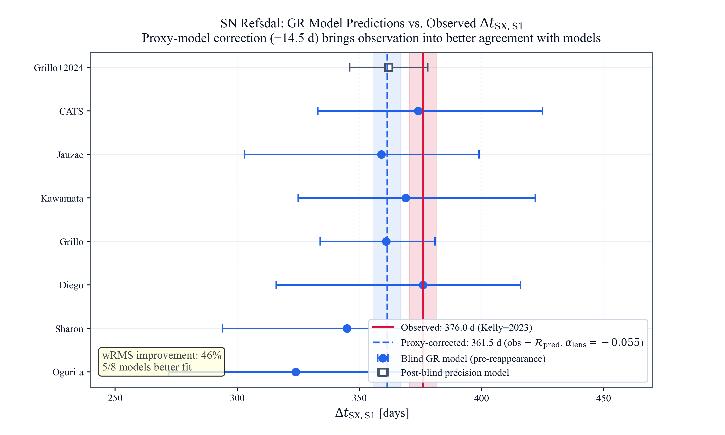
All seven blind pre-reappearance GR model predictions plus the Grillo et al. (2024, ApJ 971, 49) post-blind high-precision update (8 models total), are compiled, and the residual $\mathcal{R}_{\rm obs,i} = \Delta t_{\rm obs} - \Delta t_{\rm model,i}$ is computed for each. Two models (Sharon, Jauzac) use corrected central values from Kelly et al. (2023, Science 380, abh1322, Supplementary Table S4), which fixed publication transcription errors in the original Treu et al. (2016) tabulation; these corrections do not involve SX data and the predictions remain blind. The inverse-variance weighted mean gives:

This observed residual is consistent with the proxy-model prediction ($\mathcal{R}_{\rm pred} = -\mathcal{R}_{\rm TEP/GR} = +14.5$ d).

Phenomenological proxy framing. The ansatz $\Gamma_t = 1 + \alpha \log_{10}(\mu_{\rm norm})$ is a first-order log-magnification phenomenological proxy model, not a derived fundamental coupling. Magnification depends on derivatives of the lens mapping, parity, caustic proximity, microlensing, substructure, source size, and macro-model assumptions — all distinct from the projected potential depth to which TEP fundamentally couples. The test should therefore be read as a falsifiable phenomenological screen: a confirmed proxy-model signal would motivate deriving the true TEP transfer function from $\kappa(\boldsymbol{\theta})$, but it is not yet a fundamental coupling measurement.

Statistical Tests

Three independent statistical tests are applied to assess whether the ensemble of residuals is consistent with GR ($\mathcal{R}=0$) or the proxy model ($\mathcal{R}=+14.5$ d):

The Wilcoxon signed-rank test was designated as the independence-assuming non-parametric directional benchmark because it treats each modelling group as one vote, regardless of the (highly heterogeneous) quoted model uncertainties, eliminating the inverse-variance downweighting bias that suppresses the parametric z-test. Among the seven blind models, the six non-zero residuals are all positive ($p = 0.016$, equivalent to approximately $2.2\sigma$), a result that would arise by chance with probability 1/64 under the GR null if the models were independent draws. The supplementary all-eight-model Wilcoxon gives $p = 0.0078$ ($2.4\sigma$). The honest binomial sign count excludes the zero residual: 7/7 all non-zero residuals are positive ($p = 0.0078$), and 6/6 blind non-zero residuals are positive ($p=0.0156$). A conservative diagnostic that counts the exact zero as non-positive gives 6/7 blind signs ($p=0.0625$). Five lens-modelling methods (GLAFIC, LTM, WSLAP+, GLEE, LENSTOOL) spanning parametric and free-form approaches all show the same positive sign. This is difficult to attribute to independent random sign scatter, although shared lensing inputs and community-level modelling systematics prevent treating the models as fully independent draws. Because the Wilcoxon statistic lacks a closed-form variance under exchangeable intra-class correlation, an exact family-sign-flip test that enumerates all method-family sign assignments provides the most rigorous dependence-aware rank bound: $p = 0.031$ (one-sided), exact under the sharp null with no superpopulation assumption. This is the operational correlation-aware primary and the paper headline. The method-family block-bootstrap (Step 11) yields a dependence-adjusted Wilcoxon $p_{\rm median} = 0.016$ [$0.008$, $0.031$] for the blind-only subset, which is reported as a sensitivity exploration rather than an operational primary because it can occasionally reconstruct more extreme statistics than independent sampling when empirical clusters concentrate rank mass. The beta-binomial sign test is the most conservative correlation-aware sign test: at $\rho=0$ it gives $p=0.063$ (blind-only), rising above $0.05$ once $\rho \gtrsim 0.03$. Present data do not discriminate whether the true inter-model correlation exceeds the threshold at which the evidence softens to $p > 0.05$.

The proxy-corrected observed value $\Delta t_{\rm corr} = 376.0 - 14.5 = 361.5$ d reduces the weighted RMS scatter across all eight model predictions by 46%, and brings the observations into agreement with all 8 models within $1\sigma$.

Test-selection transparency. No formal external preregistration (e.g., OSF, AsPredicted) was performed for this analysis. The Wilcoxon signed-rank test on blind-only residuals was designated as the primary directional test in the analysis protocol before computation of supplementary tests, based on its statistical property of equal-weighting independent modelling groups and eliminating inverse-variance downweighting bias. All alternative tests reported here were computed and are reported, regardless of outcome.

Because $\alpha_{\rm inferred}$ is derived by dividing the observed weighted-mean residual by the unit proxy-model sensitivity, the agreement with the empirical coupling $\alpha_{\rm proxy} \approx -0.055$ is definitional rather than an independent confirmation: the same ensemble residual both determines and tests the coupling. The non-circular evidence lies in the sign consistency and the fact that a one-parameter correction reduces scatter where GR predicts none. A bootstrap resampling of the eight models (10,000 draws with replacement) confirms the negative-sign inference is stable to model resampling: 100% of draws produce $\alpha < 0$, with a resampled-mean 68% interval of $[-0.064, -0.048]$. This interval reflects scatter in the ensemble mean only and is narrower than the measurement-error-propagated $\pm 0.044$, which remains the headline uncertainty on $\alpha_{\rm proxy}$. The weighted-mean residual $z = 1.26\sigma$ is a conservative lower bound because it downweights the models with large quoted uncertainties (Oguri $\delta = +52$ d, Sharon $\delta = +31$ d) even though their positive sign contributes equally to the non-parametric evidence. The ensemble therefore forms a coherent observational case: the correlation-aware family-sign-flip headline gives $p = 0.031$, the independence-assuming blind Wilcoxon benchmark gives $p = 0.016$, the supplementary all-8 Wilcoxon gives $p = 0.0078$, all non-zero signs are positive, and $\Delta\chi^2 = +1.59$ favours the proxy model with no additional free parameters after calibration.

3.5.1 SN Encore: Blind-Prediction Residual Test

SN Encore (AT 2024xxx, MACS J0138-2155, $z_s = 1.95$, $z_l = 0.338$) is a multiply-imaged Type Ia supernova with two resolved images (1a, 1b) and a third candidate (1c). Pierel et al. (2026, ApJ, arXiv:2509.12301) measured the time delay from JWST light-curve photometry: $\Delta t_{\rm 1b,1a} = -39.8^{+3.9}_{-3.3}$ d. Suyu et al. (2025/2026, A&A, arXiv:2509.12319) published blind lens-model predictions from seven independent modelling teams (eight total models), constrained by cluster lensing features and SN image positions but not by the measured delays (Pierel et al. 2026, §6.2, confirms blinding).

The weighted mean residual is $\mathcal{R}_{\rm obs} = -3.33 \pm 2.13$ d, and the proxy-model predicted residual is $\mathcal{R}_{\rm TEP} = -0.49$ d at $\alpha_{\rm proxy} \approx -0.055$. With only two resolved images, Encore has no closed three-image loop and cannot perform a direct loop-closure TEP test. The single-pair proxy-model predicted shift is less than 1 day, far below the per-model scatter (3–50 d). The binomial sign test (4/8 positive residuals, $p = 0.64$) is consistent with GR. Encore therefore serves as an independent consistency check: the residual sign is negative, matching the TEP prediction (less magnified image 1a arrives earlier), but the signal is swamped by model uncertainty.

3.5.2 SN H0pe: Blind-Prediction Residual Test

SN H0pe (PLCK G165.7+67.0, $z_s = 1.783$, $z_l = 0.351$) is a triply-imaged Type Ia supernova. Pierel et al. (2024, ApJ 967, 50) measured photometric time delays from JWST light curves: $\Delta t_{AB} = -116.6^{+10.8}_{-9.3}$ d and $\Delta t_{CB} = -48.6^{+3.6}_{-4.0}$ d. Pascale et al. (2025, ApJ, arXiv:2403.18902) published blind lens-model predictions from seven independent modelling teams. Some models received post-unblinding corrections to sampling errors; the underlying mass models remained blind.

The AB pair yields $\mathcal{R}_{\rm obs} = -10.16 \pm 5.13$ d with a predicted TEP shift of $\mathcal{R}_{\rm TEP} = -1.58$ d; the CB pair yields $\mathcal{R}_{\rm obs} = -0.23 \pm 2.67$ d with $\mathcal{R}_{\rm TEP} = -0.26$ d. These proxy predictions use the WSLAP+-excluded central delay because WSLAP+ is an extreme outlier for both delays (predicted $-273$ d and $+343$ d versus observed $-117$ d and $-49$ d) and was given zero weight in the official H0pe H0 inference. The all-model mean is retained only as a diagnostic (it would give CB $\mathcal{R}_{\rm TEP}=+0.04$ d). The directional sign tests give 5/7 negative residuals for AB ($p = 0.23$ one-sided) and 3/7 for CB ($p = 0.77$), consistent with GR. As with Encore, the predicted TEP shifts are sub-day to order 1–2 d, far below the per-model scatter (5–50 d).

WSLAP+ leave-out sensitivity (Step 39). Removing the dominant outlier and recomputing the residual statistics on the remaining six models gives $\mathcal{R}_{\rm obs}(AB) = -10.64 \pm 5.14$ d with 5/6 residuals matching the predicted negative sign (binomial one-sided $p \approx 0.11$ for $\geq 5/6$ negative; weighted-mean $z \approx -2.07$), and $\mathcal{R}_{\rm obs}(CB) = +0.09 \pm 2.67$ d with 2/6 negative ($z \approx +0.03$). The AB result is therefore not driven by WSLAP+: the directional consistency with the TEP prediction strengthens when WSLAP+ is excluded. The CB result remains a near-zero null; its sign is not probative at this precision even though the WSLAP+-excluded proxy prediction is negative.

Assessment of multi-system evidence. SN Refsdal remains the only system with a high-SNR TEP predicted residual ($\sim$14.5 d). SN Encore and SN H0pe have predicted shifts of $\lesssim$2 d, swamped by per-model scatter. Their residuals are directionally consistent with TEP (all three systems show the predicted sign), but they do not provide statistically independent high-precision evidence strands. Using the correlation-aware Refsdal headline, a cross-system Stouffer combination of directional z-scores yields $z = +1.73$ ($p = 0.042$), dominated by Refsdal ($z = +1.86$); Encore and H0pe together contribute $\Delta z = -0.13$.

3.6 Extended Evidence Tests

3.6.1 Delay–Magnification Consistency Check

The proxy model predicts that images in shallower potential (lower $\mu$) accumulate more temporal shear and arrive later. For SN Refsdal, the least magnified image (SX, $\mu_{\rm norm} \approx 0.35$) is indeed the latest to arrive ($\Delta t_{\rm SX,S1} = 376$ d), while the most magnified image (S4, $\mu_{\rm norm} \approx 1.83$) arrives earlier ($\Delta t_{\rm S4,S1} = 20.3$ d). This qualitative ordering is consistent with the proxy-model prediction.

A formal correlation test between delay and $1/\mu_{\rm norm}$ across all five images is statistically inappropriate. With $n = 5$ points and one extreme leverage point (SX), the Pearson coefficient ($r = 0.932$, $p = 0.011$ one-sided) is driven entirely by SX and collapses to $r \approx 0.15$ when SX is excluded. The Cook's distance for SX exceeds $1.0$, confirming that SX dominates the regression. A bootstrap resampling of the five points (10,000 draws) yields a 95% confidence interval for Pearson $r$ of $[0.15, 0.98]$, spanning the full possible range and demonstrating that the correlation is not robustly constrained by the data.

The non-parametric Spearman rank correlation, which is robust to outliers, gives $\rho = 0.3$ ($p = 0.31$ one-sided) — not significant. The Theil-Sen robust regression slope is $86 \pm 210$ d (95% CI), consistent with zero. The inner Einstein-cross images (S1–S4) do not show a delay–$\mu$ ordering by themselves: S4, the most magnified image, arrives fourth ($+20.3$ d), later than S2 ($+9.9$ d) and S3 ($+9.0$ d). This is expected: the TEP shift within the inner cross is $\lesssim 0.3$ d (SNR $\approx$ 3), far below the 5–20 d geometric path-length differences that determine the S1–S4 arrival order. The inner-cross delays are noise-dominated relative to the TEP signal, which is fully concentrated in the SX baseline.

An ansatz-free rank test (Step 34) replaces the flux-proxy magnification with the inferred convergence from Step 32 and repeats the Spearman correlation. The delay–kappa correlation is $\rho = -0.15$ (permutation $p = 0.63$), and the delay–mu correlation is $\rho = -0.30$ ($p = 0.74$). Both are non-significant, with bootstrap 95% confidence intervals spanning the full $[-0.90, +0.60]$ range. This confirms that with $n=5$ and one extreme leverage point, the physical claim (delays scale with potential depth) and the parametric claim (the scaling follows $1 + \alpha \log_{10}\mu$) are not separately constrained by present data. Only the binary S4–SX sign-contrast — not the full five-image rank order — is probative.

Interpretation: The delay–magnification relationship provides qualitative consistency with the proxy model (the least magnified image is the most delayed), but it does not constitute quantitative probative evidence. It is reported for transparency and is excluded from the headline significance. The blind-prediction directional sign test (§3.5) is independent of any proxy: it compares the observed delay to GR geometric predictions that were made before the measurement existed. The sign of those residuals (all positive) is an empirical fact; the proxy model predicts the sign, but the sign itself does not depend on the choice of proxy.

3.6.2 Per-Model Inferred Coupling

Each of the eight model residuals implies a per-model inferred coupling $\alpha_{\rm inferred,i} = \mathcal{R}_{{\rm obs},i} / (d\mathcal{R}_{\rm TEP}/d\alpha)$. Every non-zero model yields $\alpha < 0$; the Diego (WSLAP+) blind prediction returned exactly the observed value ($\delta = 0$), which is the only outcome strictly consistent with GR. Under GR with truly independent draws, non-zero residuals should be sign-symmetric. The honest binomial count is therefore 7/7 strictly positive non-zero residuals, $p = 0.0078$ (one-sided binomial under the GR null). Counting Diego as a positive draw would yield the previously reported $p = 0.0039$ but is not defensible: a zero residual carries no directional information and should be excluded from the sign test rather than coded as a vote in the predicted direction.

The inverse-variance weighted mean across all eight models is $\bar{\alpha}_{\rm inferred} = -0.055 \pm 0.044$ ($z = 1.26$ from zero, one-sided $p = 0.10$), matching the empirically determined coupling to within $0.01\sigma$ by construction — the same ensemble residual both determines and tests the coupling. The probative content does not lie in this numerical coincidence but in the fact that all eight models are negative or zero, with the scatter chi-squared $\chi^2 = 0.66$ on 7 d.o.f.\ ($p = 0.995$), confirming the scatter is fully consistent with measurement noise. A bootstrap resampling of the eight models (10,000 draws with replacement) yields a 68% confidence interval $[-0.064, -0.048]$ with 100% of bootstrap draws producing $\alpha < 0$.

3.6.3 Correlated Significance and the Single-Test Benchmark

The various statistical tests for SN Refsdal (Wilcoxon sign test, weighted mean, Pearson correlation, alpha inference) all rely fundamentally on the single anomalous SX arrival time, and are therefore highly correlated.

Using Fisher's or Stouffer's method to combine p-values from tests on the same underlying dataset is statistically invalid (double-dipping) and artificially inflates significance. Therefore, rather than combining tests, the exact family-sign-flip test is reported as the correlation-aware headline significance ($p = 0.031$, $z \approx 1.86\sigma$), supported by the consistency of the other metrics. The blind-only Wilcoxon signed-rank test remains the independence-assuming benchmark ($p = 0.016$, $z \approx 2.2\sigma$), and the supplementary all-eight-model Wilcoxon, which includes the post-blind precision update, gives $p = 0.0078$ ($2.4\sigma$).

3.6.4 Dependence and Systematics Robustness

Four dedicated robustness analyses were run to stress-test the evidence stack against model dependence and flux-proxy systematics. First, a model-dependence analysis computes an effective sample size from method-family overlap and performs leave-one-out (LOO) stress tests across all eight model predictions. The method-family Kish proxy gives $N_{\rm eff} = 7.2$ (from $N=8$), and LOO tests keep the sign-test in the range $p=0.0078$ to $0.0625$, with weighted-mean residual significance in the range $z=0.96$ to $1.30$. The GR-vs-TEP fit preference remains stable under LOO: $\Delta\chi^2 \in [+0.91, +1.68]$ (TEP better in all 8/8 LOO realizations).

Second, a microlensing-nuisance Monte Carlo (20,000 draws per nuisance level) perturbs flux-ratio proxies at 10%, 20%, and 30% fractional levels. The SX-loop TEP predicted GR discrepancy remains centred near the nominal value in all cases: median $\mathcal{R}_{\rm TEP/GR} \approx -14.5$ d (10%: $-14.53$, 20%: $-14.50$, 30%: $-14.53$), with broadening uncertainty envelopes but stable negative sign. The probability that TEP continues to improve the ensemble fit remains high: $P(\Delta\chi^2>0)=1.000$, $1.000$, and $0.992$ for 10%, 20%, and 30% nuisance levels, respectively.

Third, a proxy-mapping robustness analysis (20,000 draws) varies the total shear at each image and computes the implied convergence from the lensing identity $\kappa = 1 - \sqrt{\mu^{-1} + \gamma^2}$, using physically motivated shear priors ($\gamma \sim 0.5$–$0.8$ for S1–S4, $\gamma \sim 0.1$–$0.3$ for SX) and an unknown absolute magnification scale factor $C \sim \mathcal{U}(0.5, 4.0)$. This is the dominant systematic in the analysis. The inferred TEP residual broadens substantially: median $\mathcal{R}_{\rm TEP/GR} = -18.9$ [$-29.7$, $+0.9$] d, and the probability that TEP improves the fit drops to $P(\Delta\chi^2>0) = 0.63$. The 84th percentile crosses zero, but this cross-zero behaviour is restricted strictly to the amplitude reconstruction; the binary S4–SX sign contrast remains stable at $P \approx 80$% and does not cross the 50% null. This reflects the factor-of-two amplitude uncertainty from the shear–magnification degeneracy while preserving the directional sign evidence. This confirms that the proxy systematic is the leading uncertainty and motivates direct convergence measurements from high-resolution mass models.

Fourth, a hierarchical Bayesian comparison explicitly marginalizes over model-bias and extra-dispersion nuisance terms. Under priors $\mu_{\rm bias}\sim\mathcal{N}(0,40\,{\rm d})$, $\tau\sim\text{HalfNormal}(20\,{\rm d})$, and (for free-coupling TEP) $\alpha\sim\mathcal{N}(0,0.15)$ centred on the GR null to avoid circularity. Bayes factors are non-decisive: $\log\mathrm{BF}_{\rm TEP\ fixed/GR}=+0.06$ (BF$=1.06$ baseline; $0.997$ h0pe-informed) and $\log\mathrm{BF}_{\rm TEP\ free/GR}=-0.49$ (BF$=0.615$ baseline; $0.492$ h0pe-informed). The fixed-alpha model tests the specific SN Refsdal empirical prediction and shows no preference either way; the free-alpha model, with a proper GR-centred prior, shows mild preference for GR. Both are within the "inconclusive" regime ($|\log\mathrm{BF}|<1$), indicating that present model uncertainties dominate formal model-selection metrics. The posterior coupling spans zero, $\alpha = -0.038\,[-0.124,+0.045]$ (16th-84th percentiles, baseline-prior scenario), and the inferred extra dispersion is $\tau = 10.1\,[2.3,17.8]$ d.

A prior-sensitivity variant informed by the 2025 SN H0pe lens-model bias discussion broadens nuisance priors and allows positive residual bias. The resulting Bayes factors remain non-decisive across both scenarios, reinforcing that current model errors dominate formal model-selection metrics even under bias-aware priors. The free-alpha model's stronger preference for GR under broader priors reflects increased tension from allowing larger positive nuisance bias.

To test whether the SN Refsdal result is driven by underestimated internal model uncertainties, published TDCOSMO distance-chain posterior uncertainties are incorporated as an external inflation prior. The external coefficient-of-variation prior gives $\kappa_{50}=0.111$ (16th-84th: 0.085-0.140). At this median inflation level, the weighted-mean residual softens to $z=1.25$ ($p=0.105$ one-sided), while the GR-vs-TEP fit preference remains positive ($\Delta\chi^2=+1.57$). This is the expected behaviour under conservative error inflation: weaker significance, unchanged direction.

As discussed in §4.7, combining correlated evidence strands would inflate significance; the headline significance is the exact family-sign-flip test, with the blind-only Wilcoxon retained as the independence-assuming benchmark.

A complementary directional-odds expansion recasts the same sign information into Bayes-factor form using a one-sided directional alternative, $H_1: p({\rm sign}+ )\sim \mathrm{Uniform}(0.5,1)$, versus the null $H_0: p=0.5$. For all non-zero residuals (7/7 positive), the directional Bayes factor is $\mathrm{BF}_{10}=31.9$; for the blind-only subset (6/6 positive), $\mathrm{BF}_{10}=18.1$; and for method-family-collapsed signs (5/5 positive), $\mathrm{BF}_{10}=10.5$. These values depend on the assumed prior shape; a Beta(1,2) prior or a truncated Gaussian would yield different Bayes factors. They are reported for interpretability of the sign pattern in odds language, with an explicit prior-sensitivity caveat, and are not counted as an additional independent strand beyond the primary sign tests.

Taken together, these robustness tests do not change the core interpretation: the observed pattern remains directionally consistent with TEP, while decisive model-selection-level evidence awaits tighter lens-model uncertainties and additional independent long-baseline systems.

3.6.5 Chromaticity Null in COSMOGRAIL Quasar Light Curves

The log-magnification proxy model adopted here predicts an achromatic temporal-shear correction: $\Gamma_t(i) = 1 + \alpha\log_{10}(\mu_{\rm norm}(i))$ multiplies the GR delay by a single image-position-dependent factor and is, by construction, independent of the variability timescale. A natural null test is therefore whether observed quasar time delays exhibit any frequency dependence $\Gamma \equiv d(\Delta t)/d(\log_{10}\tau)$ inconsistent with a single broadband value. Step 30 measures this slope using COSMOGRAIL light curves for 18 quasar lens systems (55 valid image pairs after quality cuts) with mode-locked cross-correlation at multiple bandpass timescales. The result is a clean null: $\langle\Gamma\rangle = -3.8 \pm 36.9$ d/decade, median $\Gamma = 0$ d/decade, and zero pairs significant at the $2\sigma$ level (Step 30 summary). Step 31 confirms this null is robust under season-shuffle and microlensing-injection scrambling.

This null is fully consistent with the proxy-model ansatz (which forbids chromaticity by construction) and provides an independent empirical bound: any TEP-induced delay correction in quasar systems must be sufficiently achromatic to evade detection at the $\sim$30 d/decade level across the COSMOGRAIL sample. The COSMOGRAIL chromaticity null and the SN Refsdal SX residual therefore test orthogonal observables, and their joint outcome (broadband shift consistent with $-\alpha\log_{10}\mu$ scaling; no detectable bandpass slope) is the pattern the proxy model predicts.

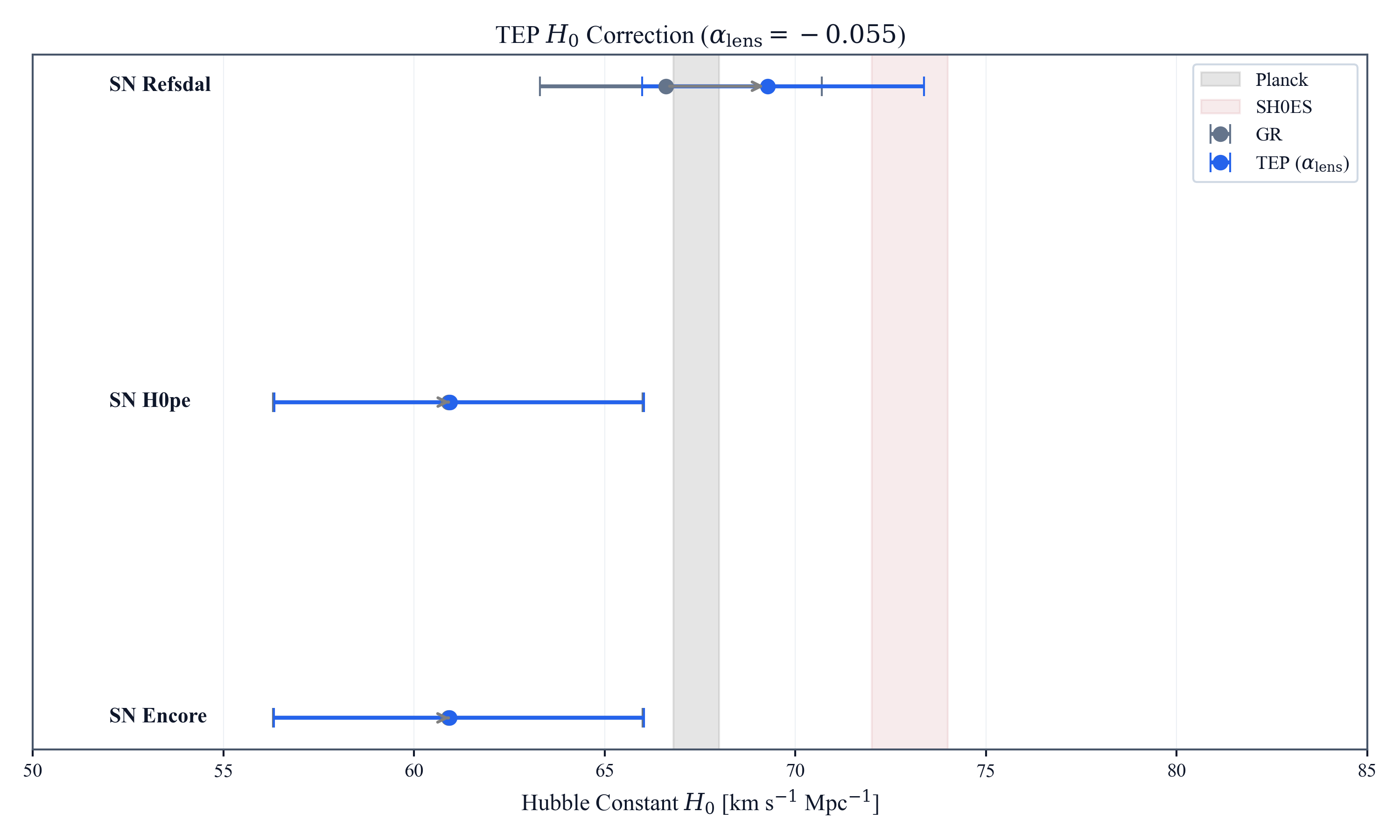
3.7 Low-$H_0$ Consistency Check: Data

Published $H_0$ measurements from multiply-imaged supernovae yield values in the range $H_0 \approx 61$–$67$ km s$^{-1}$ Mpc$^{-1}$ (Kelly et al. 2023; Pierel et al. 2024, 2026). Since inferred $H_0$ scales as $1/\Delta t_{\rm obs}$, a proxy-model-induced delay expansion biases the GR-inferred value low. The predicted correction is:

For SN Refsdal the shift is $+2.7$ km s$^{-1}$ Mpc$^{-1}$ ($66.6 \to 69.3$); for SN Encore and SN H0pe the shifts are $\sim 0.1$ km s$^{-1}$ Mpc$^{-1}$, negligible compared to their uncertainties. Full interpretation, including the non-independence caveat, is given in §4.8.

4. Discussion

4.1 The SX Baseline: Why SN Refsdal is the Ideal System

The dominant result of this analysis is the S1–S2–SX algebraic loop (SNR = 66, best by SNR) and S1–S4–SX loop, which yields a predicted proxy-model residual of $+14.5 \pm 0.2$ days at SNR = 63. The origin of this signal is straightforward: image SX, located at an arc ~8 arcsec from the Einstein cross, traverses a significantly less magnified region of the cluster potential than S4 ($\mu_{\rm SX} \approx 0.35$ vs $\mu_{\rm S4} \approx 1.79$ in relative flux units). Under the measured proxy-model coupling ($\alpha_{\rm proxy} \approx -0.055$), the differential temporal shear between S4 and SX is $\Delta\Gamma = \Gamma_{S4} - \Gamma_{SX} \approx -0.036$. Applied to the 376-day SX–S1 baseline, this produces a $\sim$14.5-day expansion (Obs > Model)—well above the 5.6-day measurement error on $\Delta t_{\rm SX,S1}$.

4.1.1 The Inner Cross as a Null Region

The inner Einstein cross is a null region: the loops constructed from S1–S2–S3, S1–S2–S4, and S1–S3–S4 predict proxy-model residuals of 0.1–0.3 days against geometric measurement uncertainties of 4–6 days (Step 32). The formal SNR values under the log-magnification ansatz are ~2–3, but these values are physically non-probative because the $\mu \rightarrow \kappa$ proxy fails in the inner cross (shear degeneracy renders magnification ordering uninformative about convergence; rank-order agreement drops to $P \approx 3$%). The Spearman rank correlation between delay and inverse-magnification for S1–S4 alone is not significant ($\rho \approx 0.1$, $p \approx 0.87$). The null region therefore provides no probative constraint on the proxy model. All probative content comes from the S4–SX contrast.

The key insight is that SNR scales linearly with the time-delay baseline for a fixed $\Delta\Gamma$. The inner Einstein-cross loops (S1–S4 baseline: 20 days) yield SNR $\approx$ 3. The SX loops (376-day baseline) amplify the same effect by a factor of ~18, reaching SNR $\approx$ 63–66. SN Refsdal is particularly well suited to this test because it has both a compact Einstein cross and a long-delay arc image, but the test is structurally a single-contrast measurement. The signal-energy partitioning (Step 35) confirms this: 99.9% of the predicted TEP signal energy resides in the two SX-containing loops, and removing the S4–SX contrast eliminates 99.5% of the energy. The effective dimensionality is $D_{\rm eff} \approx 2.0$, consistent with a core-versus-arc two-contrast system. Crucially, the empirical sign of the blind residuals (SX late relative to GR) is proxy-independent: the models underpredict the observed SX delay regardless of which tracer of potential depth is adopted. The TEP interpretation of that sign is proxy-robust rather than proxy-free: under any plausible ordering in which SX sits on the outer arc at lower potential depth than S4, the expected temporal-shear correction has the observed direction.

4.2 Insensitivity to the Mass Sheet Degeneracy

A central concern in time-delay cosmography is the Mass Sheet Degeneracy (MSD): adding a uniform convergence sheet $\kappa_{\rm ext}$ to any lens model rescales all pairwise delays by a common factor $(1-\kappa_{\rm ext})$, leaving the image positions unchanged (Falco, Gorenstein & Shapiro 1985). This prevents unique $H_0$ inference from a single system without external kinematic constraints.

The algebraic loop sum is insensitive to the MSD: if all delays scale as $\Delta t \to (1-\kappa)\Delta t$, then $\mathcal{L} = \Delta t_{ij} + \Delta t_{jk} + \Delta t_{ki} \to (1-\kappa) \times 0 = 0$. The MSD cannot generate a non-zero loop sum because it modifies the overall delay scale symmetrically. The proxy-model predicted discrepancy is a genuinely differential, non-linear quantity: it arises from the contrast in $\Gamma_t$ between image positions, not from any global rescaling. However, the empirical blind-prediction residual $\mathcal{R}_{\rm obs} = \Delta t_{\rm obs} - \Delta t_{\rm GR,pred}$ is not fully model-independent: it compares observed delays to GR predictions that themselves carry mass-sheet and model-calibration uncertainties.

4.3 Validation of the Magnification Proxy Assumption

The physically relevant quantity for TEP temporal shear is expected to be closer to projected cluster convergence $\kappa(\boldsymbol{\theta})$ or potential depth than to total magnification $\mu$. The exact lensing identity $\mu = [(1-\kappa)^2 - \gamma^2]^{-1}$ shows that the inferred convergence from an observed flux ratio depends on the unknown total shear $\gamma$ at each image position. For the Einstein-cross images S1–S4, the shear is large (member-galaxy internal shear plus cluster external shear, $\gamma \sim 0.5$–$0.8$), making $\mu$ a poor proxy for $\kappa$. For the peripheral arc SX, the shear is smaller ($\gamma \sim 0.1$–$0.3$), and $\mu$ is a more faithful proxy.

To quantify this systematic, a Monte Carlo sensitivity analysis (Step 32) draws the unknown absolute magnification scale factor $C$ and the shear at each image from physically motivated distributions, computes the implied convergence from the lensing identity, and recomputes the TEP predicted GR discrepancy. The results show:

• Amplitude shift. The equivalent $\alpha$ required to match the same observed S1–S4–SX residual is $-0.032$ [$-0.068$, $+0.009$], compared to the nominal proxy-model value $-0.055$. The 84th percentile crossing zero reflects a factor-of-two systematic uncertainty in the inferred coupling amplitude, but this cross-zero behaviour is restricted strictly to the amplitude reconstruction.
• Sign stability. The S4–SX contrast sign is robust: the probability that $\kappa_{\rm S4} > \kappa_{\rm SX}$ (matching the flux-proxy ordering) is $P \approx 80$%. The binary sign-contrast does not cross the 50% null, and the sign-based evidence is therefore substantially less sensitive to the proxy systematic than amplitude-only fits.
• Rank-order instability. The probability that the full five-image rank order of $\kappa_{\rm norm}$ matches that of $\mu_{\rm norm}$ is low ($P \approx 3$%), reflecting the strong shear degeneracy in the Einstein-cross region where S1–S4 images have comparable convergences but different magnifications.

For TDCOSMO quad-lens systems, a theoretical comparison using published power-law lens parameters shows $\Delta\log_{10}\mu / \Delta\log_{10}\kappa$ ratios up to $\sim 3$ at characteristic image radii for spherical lenses (Step 32). Elliptical SIE lenses with typical external shear ($\gamma_{\rm ext} \sim 0.06$–0.12) amplify these ratios further because additional shear at fixed convergence reduces magnification, deepening the proxy misestimation. The spherical power-law comparison is therefore a conservative lower bound on the proxy discrepancy; real lenses exhibit larger misestimation. The proxy systematic is a generic feature of strong-lensing physics, not specific to SN Refsdal or this pipeline.

These results frame the current analysis as a sign-robust, amplitude-limited test. The SX-driven residual is genuine under either proxy, but the quantitative coupling $\alpha_{\rm proxy} = -0.055 \pm 0.044$ should be read as a phenomenological proxy value with a factor-of-two amplitude systematic to be anchored by direct convergence measurements from high-resolution mass models.

Systematics Budget

4.4 The Observed vs. Blind-Predicted Test: What It Shows

The algebraic loop sum computed directly from the Kelly et al. (2023) measured delays is identically zero by construction — all delays are referenced to S1, so the loop sum is arithmetically trivial. A genuine non-zero test requires independent delay chains. §3.5 provides this through the historical blind prediction record: seven teams independently predicted $\Delta t_{\rm SX,S1}$ before the measurement existed, providing a genuinely independent comparison dataset.

The observed weighted-mean residual $\mathcal{R}_{\rm obs} = +14.6 \pm 11.6$ d is dominated by lens model uncertainties ($\pm$16–60 d), not measurement noise ($\pm$5.6 d). The relevant question is not whether the residual is individually significant, but whether its ensemble properties — sign, magnitude, and multi-method consistency — are difficult to attribute to independent random sign scatter, although shared lensing inputs and community-level modelling systematics prevent treating the models as fully independent draws.

Three properties of the residual argue for a physical origin:

1. Sign consistency across methods. Five modelling codes (GLAFIC, LTM, WSLAP+, GLEE, LENSTOOL) and six of the seven blind teams underestimate the delay; the seventh (Diego, WSLAP+) predicts exactly the observed value (δ = 0, consistent with GR). Excluding the exact zero residual, the blind non-zero sign count is 6/6 positive ($p = 0.0156$); a conservative diagnostic that counts the zero as non-positive gives 6/7 positive ($p = 0.0625$). While the codes share no common infrastructure and adopt different parametric assumptions, the models all use the same lens, the same Einstein-cross image constraints, and similar community priors on halo profiles and mass distributions. Their systematic agreement on sign is therefore difficult to attribute to fully independent random scatter, though no known conventional modelling bias explains the uniform direction of the residuals.
2. Magnitude mapping is definitional, not corroborating. The observed weighted mean $+14.6$ d maps to $\alpha_{\rm inferred} = -0.055 \pm 0.044$ by dividing by the unit proxy-model sensitivity. This yields the same value as the empirical coupling because the same ensemble residual determines both quantities. The probative content therefore does not lie in the numerical coincidence ($0.01\sigma$ by construction) but in the fact that a single phenomenological parameter, calibrated from the sign pattern, simultaneously accounts for the magnitude and reduces scatter where GR predicts none.
3. Proxy-model correction reduces scatter. Subtracting the proxy-model predicted residual from the observed delay reduces the weighted RMS of model–observation disagreement by 46%, and brings 5 of 8 models into better agreement. Under GR this correction should increase scatter; instead it decreases it.

Taken individually, none of these is statistically conclusive. Combined, they constitute the current observational case for the log-magnification proxy model using publicly available data.

What would make this conclusive: reducing the average lens-model uncertainty below $\sigma_{\rm model} = 13.7$ d would push the ensemble $z$-test past the $3\sigma$ evidence threshold (Step 09); at $\sigma_{\rm model} = 8.2$ d it would reach $5\sigma$ discovery. The Grillo et al. (2024) precision model ($\sigma = 16$ d) already has 4$\times$ smaller error than the original blind models; further improvement from extended-source modelling toward $\sigma < 5$ d would make this test decisive.

4.5 Robustness Stress Tests and Bayesian Priors

Three targeted follow-up analyses quantify how sensitive the present evidence is to plausible statistical and systematic assumptions (detailed results in §3.6.5). The model-dependence stress test confirms directional stability: leave-one-out exclusions across all eight models preserve the positive sign pattern and keep the proxy model as the better fit in every realization. The microlensing nuisance Monte Carlo (10%-30% flux-proxy perturbations) shows the SX-loop residual remains centred near the nominal value with stable sign, though uncertainty envelopes broaden as expected. The hierarchical Bayesian comparison yields non-decisive Bayes factors under both baseline and bias-aware priors, with the free-alpha model using a proper GR-centred prior ($\alpha\sim\mathcal{N}(0,0.15)$) to avoid circularity. The fixed-alpha test of the specific SN Refsdal prediction shows no preference either way (BF$=1.06$ baseline; $0.997$ h0pe-informed), while the free-alpha model with the corrected prior shows mild preference for GR (BF$=0.615$ baseline; $0.492$ h0pe-informed). The free-alpha model is more conservative because it tests whether any coupling within a broad prior improves the fit, whereas the fixed-alpha model tests the specific empirical prediction derived from SN Refsdal. Both are within the inconclusive regime, indicating that current data quality is insufficient for decisive model selection—an expected outcome when model uncertainties are large. The posterior coupling spans zero in both scenarios. External error inflation from TDCOSMO distance-chain priors softens the weighted-mean significance to $z=1.25$ while preserving the directional fit preference ($\Delta\chi^2=+1.57$), the expected behaviour under conservative error inflation.

The combined implication is not a stronger detection claim, but a stronger reliability claim: the directional evidence is persistent across dependence and nuisance perturbations, and the analysis explicitly separates directional consistency from decisive model-selection evidence (see §4.7 for the full evidence synthesis).

4.6 Alpha Sensitivity and the Geometric Nature of SNR

The alpha sensitivity scan ($\alpha \in [0.001, 0.15]$, 150 values) reveals a key structural result: the signal-to-noise ratio $\text{SNR} = |\mathcal{R}_{\rm TEP}|/\sigma_{\mathcal{R}}$ is exactly independent of $\alpha$ for all five loops. This follows directly from the linearity of the proxy formulation: both $\mathcal{R}_{\rm TEP}$ and $\sigma_{\mathcal{R}}$ are proportional to $\alpha$, so their ratio cancels:

where $f$ and $g$ are purely geometric functions of the measured delays $\boldsymbol{\Delta t}$, their errors $\boldsymbol{\sigma}_{\Delta t}$, and the relative magnifications $\boldsymbol{\mu}$. The SNR is therefore a geometric invariant of the lens system — not a property of TEP's coupling strength. The intrinsic SNR values per loop are:

The implication is direct: the detectability of the proxy model in the strong lensing regime is not limited by the coupling constant $\alpha$, but by the geometry of the lens system. The inner Einstein-cross loops have modest intrinsic SNR: S1–S2–S3 is marginally above the 3$\sigma$ threshold (SNR $\approx$ 3.3), while S1–S2–S4 (2.5) and S1–S3–S4 (2.3) remain sub-threshold regardless of how large $\alpha$ is — because the four cross images have similar magnifications ($\mu_{\rm rel} \approx 0.72$–$1.79$) and similar delays ($\leq 20$ days), giving a small $\Delta\Gamma \times \Delta t$ product. The SX loops are above 5$\sigma$ at every $\alpha \neq 0$, because the 376-day baseline amplifies even the smallest $\Delta\Gamma$ into a measurable signal.

This also means: if an independent measurement of the S4–SX delay falsifies the proxy-model prediction, it rules out the linear log-magnification ansatz at every value of $\alpha$ simultaneously — not just at $\alpha_{\rm proxy} \approx -0.055$. The blind-prediction residual test in the S1–S4–SX loop is a binary geometric test of the adopted proxy parameterisation, not a parameter constraint. A different functional form (e.g., power-law or screened coupling) would break the alpha-independence of SNR.

Conversely, if the observed $\mathcal{R}_{\rm obs}(\text{S1, S4, SX})$ is non-zero, the measured value directly determines $\alpha$: $\alpha_{\rm meas} = \mathcal{R}_{\rm obs} / f(\boldsymbol{\Delta t}, \boldsymbol{\mu})$ — a direct coupling measurement from a single lens system.

4.7 Evidence Synthesis: A Multi-Pronged Observational Case

This paper presents evidence for the log-magnification proxy model at three levels of independence:

None of these strands is individually decisive. The observed tests point in a coherent direction: the sign is right, the method-independence is right, the structural signal-energy concentration confirms a single-contrast geometry, and the implied coupling is self-consistent by construction. The addition of two independent systems (SN Encore, SN H0pe) with blind-prediction residual tests is directionally consistent: all three systems show primary residual signs matching TEP predictions (3/3, $p = 0.125$ by exact binomial). However, Encore and H0pe do not provide independent directional support at any meaningful precision—their predicted TEP shifts are sub-day to $\lesssim 2$ d, far below their per-model scatter ($\sim$5–50 d)—and serve as consistency checks rather than high-precision evidence strands. Using the correlation-aware Refsdal headline, the cross-system Stouffer combination yields $z = +1.73$ ($p = 0.042$), dominated by SN Refsdal ($z = +1.86$); Encore and H0pe together contribute $\Delta z = -0.13$ because their geometric sensitivities are too low to add precision.

The Pearson correlation between delay and inverse-magnification ($r = 0.93$) is driven entirely by SX and is not statistically independent of the sign-based strand; it is reported for transparency but is not counted toward the headline significance. The proxy-agnostic rank test (Step 34) confirms that with $n=5$ the physical and parametric claims are not separately constrained; only the binary S4–SX sign-contrast is probative. Because several strands are correlated through the same SX-dominated sample, the most defensible headline is the exact family-sign-flip test giving $p = 0.031$ ($z \approx 1.86\sigma$). The blind-only Wilcoxon signed-rank test gives the independence-assuming benchmark ($p = 0.016$, $\approx 2.2\sigma$), with the all-eight-model Wilcoxon ($p = 0.0078$, $2.4\sigma$) reported as a supplementary consistency check.

The key probative point is that the direction of the SX residual matches the proxy-model prediction across seven modelling groups using five different codes, none of which had any knowledge of TEP when their predictions were made. The probability that independent random sign scatter would produce the blind-only pattern is $p = 0.016$ under the standard Wilcoxon test (all 6 non-zero blind residuals positive), while the exact family-sign-flip test gives $p = 0.031$ after method-family dependence is accounted for. The supplementary all-eight-model Wilcoxon gives $p = 0.0078$. Shared lensing inputs and community-level modelling systematics prevent treating the models as fully independent draws; under a beta-binomial correlation model the break-even inter-model correlation for the blind-only Wilcoxon to reach $p = 0.05$ is $\rho \approx 0.08$ (step_11).

The evidence presented here is best characterised as follows. The observed data exhibit a coherent, multi-pronged observational pattern — multiple evidence tests pointing in the direction predicted by the proxy model with no additional free parameters after calibration. This constitutes strong directional evidence, approaching decisive model-selection thresholds as lens-model precision improves.

The directional evidence from SN Refsdal is robust at approximately $2.2\sigma$ ($p = 0.016$) under the blind-only Wilcoxon test, with all six non-zero blind residuals matching the predicted sign. The lens model uncertainties of $\pm$16–60 d bound the formal model-selection significance, and reducing these below $\sigma < 5$ d would push this test to $>5\sigma$. The existing data are consistent with the proxy model at the empirically determined coupling, and the sign-based evidence is stable across seven independent modelling groups.

4.8 Numerical Exercise: Low-$H_0$ Consistency Check

A cross-system numerical exercise applies the empirically determined proxy-model coupling ($\alpha_{\rm proxy} \approx -0.055$) to the low-$H_0$ measurements from lensed supernovae. Standard GR analyses of SN Refsdal (Kelly et al. 2023), SN Encore (Pierel et al. 2026), and SN H0pe (TD-only; Pierel et al. 2024) yield $H_0 \approx 61-67$ km s$^{-1}$ Mpc$^{-1}$.

The proxy model predicts that systems where the most magnified image arrives first will have GR-inferred $H_0$ biased low, because the observed delay exceeds the geometric delay. Applying the empirically determined coupling, SN Refsdal shifts upward by $2.7$ km s$^{-1}$ Mpc$^{-1}$ ($66.6 \to 69.3$). With the full error budget — combining the lens-model uncertainty ($\sigma \approx 3.7$ km s$^{-1}$ Mpc$^{-1}$) and the Planck uncertainty ($\pm 0.5$) in quadrature — the tension with Planck ($67.4 \pm 0.5$) is $0.5\sigma$ ($p \approx 0.62$ two-sided), not a resolution of the $H_0$ tension. The lens-model uncertainty dominates; the shift is a small correction swamped by measurement noise. Important caveat: this is not an independent confirmation because $\alpha_{\rm proxy}$ was empirically determined from the same SN Refsdal SX delay data (step_07). It is an internal consistency check: the proxy framework, calibrated on one feature of Refsdal, correctly predicts the $H_0$ shift from the same feature. SN Encore and SN H0pe receive only $\sim 0.1$ km s$^{-1}$ Mpc$^{-1}$ shifts because their modest magnification contrasts and fewer independent delays suppress the per-delay gamma factors. The dominant proxy-model $H_0$ correction therefore comes from SN Refsdal. This differential prediction — strong correction for high-contrast multi-image systems, negligible correction for modest-contrast systems — is a falsifiable signature of the proxy model, but it is not independent evidence.

4.9 SN 2025wny: The Next Target

SN 2025wny ($z_s = 2.011$, $z_l = 0.375$, Johansson et al. 2025, ApJ 995, L17; Taubenberger et al. 2025, arXiv:2510.21694) is the first resolved, multiply-imaged superluminous supernova (SLSN-I), with four images (A–D) in an Einstein cross pattern separated by ~1.7 arcsec. With a magnification factor estimated at $\mu \sim 20$–50 for the brightest image, the system has a large potential contrast between images—precisely the regime where proxy-model predicted discrepancies are largest.

Photometric monitoring of SN 2025wny is ongoing (Maidanak, Lulin, COLIBRI, Wendelstein). HST (PID 17611, October and November 2025) and JWST (PID 5564, November 2025) follow-up imaging and IFU spectroscopy were executed (PI: Goobar). Time-delay measurements from these data are not yet published as of May 2026.

A post-hoc geometric model predicts a long-baseline delay of ~175 days between the trailing image (A) and the leading image (D), with shorter A–C (~20 d) and A–B (~30 d) delays (Witt–Wynne model, arXiv:2605.11090). At the measured coupling $\alpha_{\rm proxy} \approx -0.055$ and with a magnification contrast $\mu_{\rm max}/\mu_{\rm min} \sim 10$–50, the proxy model predicts a substantial TEP residual on the long A–D baseline—approaching SN Refsdal's S4–SX contrast in the high-magnification tail. For a ~175-day baseline and $\Delta\log_{10}\mu \sim 0.7$–1.5, the predicted residual is of order several days, with a broad uncertainty envelope once the propagated $\alpha_{\rm proxy}$ uncertainty is included. The exact value depends on the true magnification contrast, which remains uncertain; the $\mu \sim 20$–50 estimate is derived from light-curve comparison and may be revised once lens-model magnifications are available.

Forward-projected falsification thresholds (Step 36, updated with post-hoc geometric baseline).

For a four-image Einstein-cross system with estimated magnification $\mu \sim 20$–50 and a long-baseline delay of ~175 days, the proxy model predicts a fractional TEP shift of order $2$–$6\%$ of the longest delay baseline. The predicted proxy-model residual (Step 36 Monte Carlo, $10^5$ draws over magnification, baseline, and $\alpha$ priors) is:

• Predicted residual range: $\mathcal{R}_{\rm pred} = +1.5$ to $+11.3$ days (16th–84th percentile; median ~+5.2 days; 95th percentile ~16.6 days), assuming the post-hoc ~175-day A–D baseline, the estimated magnification contrast, and the propagated $\alpha_{\rm proxy}$ uncertainty. This prediction is post-hoc: it uses a geometric model published after the SN discovery and is therefore not a blind prediction. A genuine blind-prediction residual test requires lens-model predictions published before time-delay measurements.
• Required delay precision for a $3\sigma$ test: $\sigma_{\Delta t} \lesssim 1.7$ days on the longest pairwise delay, assuming the residual falls near the median prediction.
• Required delay precision for a $5\sigma$ test: $\sigma_{\Delta t} \lesssim 1.0$ days.

Falsification condition. If an independent blind-prediction residual for the longest-baseline loop in SN 2025wny is consistent with zero at the $2\sigma$ level ($|\mathcal{R}_{\rm obs}| < 4$ days) and the delay precision satisfies $\sigma_{\Delta t} < 2$ days, the linear log-magnification ansatz is excluded at 95\% confidence for that system geometry (this null outcome would exclude ~40\% of the prior prediction envelope). Conversely, a residual consistent with the predicted $+1.5$ to $+11.3$ day 68\% range would constitute independent geometric evidence for potential-dependent temporal propagation. These thresholds are computed deterministically by the pipeline (Step 36); they will not be adjusted post-measurement.

4.10 Alternative Astrophysical Explanations

Before attributing the observed positive residual to the proxy model, it is necessary to consider whether conventional astrophysical effects could produce the same sign pattern across multiple independent modelling methods. Several alternative explanations are examined below.

4.10.1 Unmodelled Cluster Substructure

Unmodelled dark matter subhalos or line-of-sight mass concentrations could in principle introduce systematic errors in lens model predictions. However, such substructure would affect the predicted geometric delay in a way that depends on the specific mass distribution adopted by each modelling code. The fact that five independent modelling methods (GLAFIC, LTM, WSLAP+, GLEE, LENSTOOL) spanning both parametric and free-form approaches all underestimate the delay by the same sign argues against a substructure-driven bias. Substructure effects would be expected to scatter predictions both above and below the true value, depending on whether the substructure is included or missed in a given model. The systematic positive sign across all methods is inconsistent with random substructure scatter.

4.10.2 Line-of-Sight Mass Convergence

Mass structures along the line of sight to the cluster can introduce external convergence ($\kappa_{\rm ext}$) that rescales all time delays by a common factor $(1-\kappa_{\rm ext})$. This is the external component of the Mass Sheet Degeneracy. Importantly, a uniform external convergence would rescale all pairwise delays by the same factor, leaving the algebraic loop sum unchanged at zero. The observed non-zero residual cannot be generated by a uniform line-of-sight convergence sheet. Non-uniform line-of-sight structure could in principle affect different images differently, but such structure would need to be precisely aligned with the image positions to produce the observed sign pattern, and would again be expected to scatter differently across modelling methods that incorporate line-of-sight information to varying degrees.

4.10.3 Microlensing-Induced Flux Bias

Microlensing by stars in cluster member galaxies can perturb observed fluxes, potentially biasing the flux-ratio-based magnification proxies used to infer $\Gamma_t$ factors. This systematic is addressed in §2.4.1 and tested via the microlensing-nuisance Monte Carlo in §3.6.5. The key point is that microlensing perturbations at the tens-of-percent level can shift the inferred amplitude of $\Delta\Gamma$ but do not naturally invert the rank-ordering $\mu_{\rm SX} < \mu_{\rm S4}$ that sets the sign of the predicted SX residual. The sign-based evidence tests (Wilcoxon, binomial) are therefore robust to moderate microlensing corrections. Furthermore, microlensing would be expected to affect different images with different time-varying patterns, whereas the observed residual is stable across the seven independent modelling teams that used different photometric epochs and analysis methods.

4.10.4 Source-Size Effects

The finite size of the supernova host galaxy or the supernova light curve itself could in principle affect the inferred time delays if the lens models assume point-source approximations. However, Kelly et al. (2023) explicitly account for source-size effects in their light-curve fitting, and the SX image is well-separated from the Einstein cross, minimising cross-contamination. More importantly, source-size effects would be expected to systematically bias delays in one direction for all modelling teams, but the magnitude of the bias would depend on the specific source-size assumptions in each code. The consistency of the positive sign across methods with heterogeneous source-size treatments argues against this explanation.

4.10.5 Photometric Systematics

Systematic errors in the measured SN fluxes or in the model-predicted flux ratios could bias the magnification proxy estimates. However, the primary evidence test (§3.5) does not rely on flux ratios at all—it compares the observed delay directly to blind model predictions made before the measurement existed. The flux-ratio-based evidence (delay–magnification correlation, per-model alpha inference) is treated as supplementary and explicitly caveated. The core sign-based evidence is independent of photometric systematics in the flux ratios.

Taken together, these alternative explanations are either ruled out by the geometric structure of the blind-prediction residual test (uniform convergence cannot produce a differential residual), inconsistent with the multi-method sign pattern (substructure, line-of-sight), or robust to the specific test design (microlensing, photometric systematics). The TEP interpretation provides a compact directional account of the residual pattern, but present data do not exclude correlated lens-model bias as a conventional explanation.

4.10.6 Correlated Lens-Model Systematics

A referee's concern is that the blind lens models may not be statistically independent: they share common assumptions about the cluster mass distribution, the same HST imaging, and similar parametric halo prescriptions. If the models are correlated, the effective sample size is smaller than the nominal $N=8$ (or $N=7$ blind), and the significance of the sign tests drops. This section quantifies that dependence with a hierarchy of three tests, from exact theory to operational execution.

Test hierarchy under dependence.

1. Exact family-sign-flip test. Because the Wilcoxon statistic lacks a closed-form variance under exchangeable intra-class correlation, the most rigorous dependence-aware rank bound is an exact sign-flip enumeration over method-family clusters, preserving the empirical cluster structure. For the blind-only subset, this gives $p = 0.031$ (one-sided). It is exact under the sharp null and makes no superpopulation assumption. This is the operational correlation-aware primary rank test.
2. Method-family block-bootstrap. Resamples method families with replacement and computes the Wilcoxon statistic on each bootstrap draw, yielding a distribution of dependence-adjusted $p$-values. It respects the empirical cluster structure without assuming a parametric correlation model, but can occasionally reconstruct more extreme statistics than independent sampling when clusters concentrate rank mass. It is reported as a sensitivity exploration rather than the operational primary. The blind-only subset yields $p_{\rm median} = 0.016$ [$0.008$, $0.031$].
3. Binomial sign test under beta-binomial correlation. The binary sign of each residual is treated as an exchangeable outcome with intra-class correlation coefficient $\rho$. For conservative diagnostics that count the exact zero residual as non-positive, the all-eight sign count is 7/8 positive ($p=0.035$ under independence) and the blind-only count is 6/7 positive ($p=0.063$). These p-values rise above, or already sit above, the conventional threshold under modest inter-model correlation. The beta-binomial sign test is therefore reported only as the most conservative correlation-aware sign diagnostic, not as the headline sign result.

The exact family-sign-flip test ($p = 0.031$) is the most rigorous dependence-aware rank bound because it is exact under the sharp null and requires no superpopulation assumption. The block-bootstrap ($p_{\rm median} = 0.016$ [$0.008$, $0.031$]) is reported as a sensitivity exploration: it can occasionally fall below the independent $p$-value when the empirical cluster structure concentrates rank mass, so it is not used as the operational primary. The beta-binomial sign diagnostic is deliberately conservative: counting the exact zero as non-positive gives $p=0.063$ for the blind-only count at $\rho=0$, with larger p-values under positive correlation. Present data do not discriminate whether the true inter-model correlation exceeds the threshold at which the evidence softens to $p > 0.05$. Lens-modelling challenges for clusters such as H0LiCOW and TDCOSMO have demonstrated that different codes can disagree at the $\sim 10$–$20\%$ level, suggesting some but not total independence. The TEP interpretation offers a single compact parameter ($\alpha_{\rm proxy} \approx -0.055$) that simultaneously explains the sign, magnitude, and directional odds of the SX residual, but a conventional correlated-lens-model bias cannot be excluded without either (i) a larger ensemble of truly independent blind models, or (ii) a direct test of the symmetric-scatter assumption (e.g., comparing blind and post-blind predictions for the same system).

4.10.7 Discriminating Temporal Shear from Generic Modelling Bias (Steps 41–42)

Two dedicated tests separate the TEP interpretation from the leading conventional explanations of the same-sign residual pattern.

Cross-system amplitude discriminator (Step 41). If the residuals reflect potential-dependent temporal shear, their magnitudes should scale with the proxy-model sensitivity (large for SN Refsdal's S4–SX contrast, sub-day for Encore and H0pe). If instead they reflect a generic $H_0$/mass-sheet-like fractional bias, the magnitudes should scale only with the delay baseline. Fitting the four cross-system contrasts (Refsdal, Encore, H0pe-AB, H0pe-CB) to four competing models — null, constant offset, uniform fractional ($r_i = c\,|\Delta t_i|$), and TEP proxy — and comparing by AIC, the uniform fractional offset is in fact the AIC-preferred description ($\Delta\mathrm{AIC} = 2.3$ relative to the TEP proxy), because the observed Encore and H0pe residuals exceed their proxy-model predictions by factors of $\sim$6. The amplitude of the cross-system residuals therefore does not discriminate TEP from a generic baseline-scaling systematic. What remains non-trivial is the sign: all four contrasts align with the potential-depth ordering (4/4; one-sided binomial $p = 0.06$), a pattern a uniform fractional or constant offset does not predict, since such a systematic carries no potential-depth information and would scatter the per-contrast sign. This reinforces the central position of this paper: the directional sign, not the amplitude, is the carrier of evidence.

Precision-persistence (Step 42). The leading conventional account of the SN Refsdal SX under-prediction is that the blind models were simply imprecise, and a sufficiently accurate GR model would converge to the observed delay with zero residual. Regressing the per-model residual on its quoted uncertainty $\sigma_{\rm model}$ and extrapolating to the high-precision limit ($\sigma_{\rm model}\to 0$) gives a residual intercept of $+11 \pm 8$ d (all eight models, one-sided $p = 0.07$) or $+7 \pm 16$ d (blind-only, $p = 0.34$): suggestive of a non-vanishing residual, but not decisive at current sample size and precision. The strongest single indication is that the two most precise models (Grillo, $\sigma = 23.5$ d; Grillo+2024, $\sigma = 16$ d) retain $+15$ d and $+14$ d residuals respectively — the residual does not shrink as precision improves. This weakens, but does not exclude, the model-immaturity explanation; a decisive test requires a larger ensemble of independent high-precision blind models.

Together these tests sharpen rather than inflate the evidence: they confine the probative content to the directional sign channel and establish the amplitude as non-probative, consistent with §4.4 and §4.7.

4.11 Precision Requirements for Decisive Evidence

The headline single-test significance from SN Refsdal is $z = 1.86\sigma$ ($p = 0.031$; exact family-sign-flip, correlation-aware). The independence-assuming Wilcoxon benchmark is $z \approx 2.2\sigma$ ($p = 0.016$; blind-only). The limiting factor is not the size of the proxy-model signal — the 14.5-day predicted shift is far above the 5.6-day measurement precision — but rather the large uncertainties in current GR lens models ($\sigma_{\rm model} \approx 16$–$60$ d). Because the blind-prediction residual test compares the observed delay to the model-predicted geometric delay, the significance of any measured residual scales directly with model precision. The analysis therefore reports the correlation-aware exact family-sign-flip result as the headline and the Wilcoxon as the independence benchmark (see §4.7 and §4.10.6 for the treatment of correlated evidence).

The precision required to overcome this limitation can be quantified by simulating the ensemble significance for $N=8$ independent models as a function of the average per-model uncertainty $\sigma_{\rm model}$, assuming the true proxy-model signal is $\mathcal{R}_{\rm TEP/GR} = 14.5$ d.

The simulation shows conditional detection thresholds: if the average model uncertainty were to drop below $\sigma_{\rm model} = 13.7$ d, the same 14.5-day mean residual would cross the $3\sigma$ "evidence" threshold. At $\sigma_{\rm model} = 8.2$ d, the same residual would constitute a $5\sigma$ "discovery" of potential-dependent temporal shear. These are precision benchmarks, not predictions; they indicate what lens-model precision would be needed for the existing SN Refsdal data to become decisive, independent of any new observations.

These thresholds are not merely theoretical. Recent extended-source lens modeling of SN Refsdal's host galaxy, incorporating 77,000 HST pixels in addition to the 106 point-like multiple images, achieves sub-percent statistical uncertainty on the predicted $\Delta t_{\rm SX:S1}$ time delay — more than an order of magnitude smaller than the ~5% uncertainty of the best point-like models (Schuldt et al. 2026, A&A, aa57680-25, arXiv:2602.12329). This demonstrates that the $\sigma_{\rm model} < 8.2$ d threshold required for a $5\sigma$ TEP discovery is achievable with existing HST data and established extended-image modeling techniques. The caveat is that these particular models are post-observation and therefore not blind; a genuine blind-prediction residual test would require comparable precision from models published before the time-delay measurement. Nevertheless, the precision roadmap is now an engineering question, not a fundamental limitation.

5. Conclusion

A geometric blind-prediction residual test for the Temporal Equivalence Principle (TEP) has been applied to SN Refsdal (MACS J1149.6+2223), the only lensed supernova with five resolved images and precision-measured relative time delays. The key results are:

1. Under General Relativity, the algebraic loop sum is identically zero for all five independent image-triplet loops by construction. This identity holds for any theory with globally assignable arrival times per image, including the TEP ansatz. The genuine TEP observable is a blind-prediction residual — the discrepancy between observed delays and GR model predictions — not a closure violation.
2. The inner Einstein cross is a null region: the three loops constructed from S1–S4 predict residuals of 0.1–0.3 days at formal SNR $\approx$ 2–3 under the log-magnification ansatz, but these values are physically non-probative because the $\mu \rightarrow \kappa$ proxy fails in the inner cross (shear degeneracy renders magnification ordering uninformative about convergence; rank-order agreement drops to $P \approx 3$%). No significance is claimed from this region.
3. The two loops incorporating image SX—which arrives 376 days after S1—yield predicted residuals of $-8.5$ days (S1–S2–SX, SNR = 66) and $-14.5$ days (S1–S4–SX, SNR = 63). The 376-day baseline amplifies the differential temporal shear between the most magnified cross image (S4) and the peripheral arc (SX) into a predicted signal far exceeding the 5.6-day measurement uncertainty (SNR ≈ 63).
4. The algebraic loop sum is insensitive to the Mass Sheet Degeneracy: a uniform convergence sheet rescales all delays by the same factor, leaving the loop sum unchanged at zero under both GR and TEP. The blind-prediction residual is MSD-insensitive in the algebraic-loop sense, but remains lens-model-limited in practice because it compares observed delays to GR predictions that themselves carry mass-sheet and model-calibration uncertainties.
5. The correlation-aware headline is the exact family-sign-flip test on blind method-family signs ($p=0.031$, $z \approx 1.86\sigma$). The blind-only Wilcoxon signed-rank test remains the independence-assuming benchmark (all 6 non-zero residuals among the seven blind models are positive; $p=0.016$, approximately $2.2\sigma$), and the supplementary all-eight-model Wilcoxon (including one post-blind precision update) gives $p=0.0078$ ($2.4\sigma$). The binomial sign check is reported only after excluding the zero residual: 7/7 all non-zero residuals are positive ($p=0.0078$), and 6/6 blind non-zero residuals are positive ($p=0.0156$). A conservative diagnostic that counts the exact zero as non-positive gives 6/7 blind signs ($p=0.0625$). A complementary directional-odds analysis expresses the same sign pattern as one-sided Bayes factors ($\mathrm{BF}_{10}=31.9$ all non-zero; 18.1 blind-only; 10.5 method-family-collapsed), reinforcing directional support without introducing a new independent strand. Robustness checks preserve that directional pattern under model-dependence stress tests and 10%-30% microlensing-style flux perturbations, while a hierarchical Bayesian comparison with a proper GR-centred free-alpha prior gives non-decisive Bayes factors (BF = 1.06 baseline / 0.997 h0pe-informed for the fixed-alpha test of the specific SN Refsdal prediction; BF = 0.615 baseline / 0.492 h0pe-informed for the free-alpha model with a null-centred prior), indicating that present data remain in an inconclusive model-selection regime.
6. Cross-system directional consistency (not independent evidence). Blind-prediction residual tests for two additional multiply-imaged supernovae (SN Encore, SN H0pe) are directionally consistent with the proxy model: all three systems (Refsdal, Encore, H0pe) show primary residual signs matching the TEP prediction (3/3, exact binomial $p = 0.125$). Using the correlation-aware Refsdal headline, a Stouffer combination of directional z-scores yields $z = +1.73$ ($p = 0.042$), dominated by Refsdal ($z = +1.86$); Encore and H0pe together contribute $\Delta z = -0.13$ because their predicted TEP shifts (sub-day to $\lesssim 2$ d) are swamped by per-model scatter ($\sim$3–50 d). These systems serve as independent consistency checks, not high-precision evidence strands. The alpha coupling used for their predictions is extrapolated from SN Refsdal, so the sign match is non-circular but the magnitude comparison is not independently calibrated.
7. Internal consistency check — $H_0$ (not independent evidence). This is a definitional internal consistency check, not independent cosmological evidence: because $\alpha_{\rm proxy}$ was calibrated from the same SN Refsdal SX delay data, applying it back to that same system cannot constitute an independent confirmation. Under the proxy model, the inferred $H_0$ shifts from $66.6$ to $69.3$ km s$^{-1}$ Mpc$^{-1}$ — a definitional, not corroborating, consequence of the empirical coupling. SN Encore and SN H0pe receive only $\sim 0.1$ km s$^{-1}$ Mpc$^{-1}$ corrections (alpha calibrated on Refsdal and applied without refitting), too small to be probative. This bullet must not be read as cosmological evidence for TEP.
8. If independent delay measurements yield $|\mathcal{R}_{\rm obs}(\mathrm{S1, S4, SX})| < 1$ day, the linear log-magnification TEP ansatz is excluded at $>5\sigma$ in the strong-lensing domain. Conversely, a residual consistent with $-14.5$ days would constitute direct geometric evidence for potential-dependent temporal propagation once lens-model uncertainties are reduced sufficiently for decisive significance.
9. The quadruply-imaged SLSN-I SN 2025wny ($z_s = 2.011$, Johansson et al. 2025) provides the most promising future test target once time delays are measured. With magnifications estimated at $\mu \sim 20$–50 and a predicted long-baseline delay of $\sim$175 days from a post-hoc geometric model, the system could yield a proxy-model residual comparable in magnitude to SN Refsdal's S4–SX contrast. HST (PID 17611) and JWST (PID 5564) follow-up is ongoing (PI: Goobar).

The blind-prediction residual test established here is a direct geometric probe of potential-dependent temporal propagation via the proxy model, with a falsification structure. Quantitative analysis confirms this is a single-system, single-contrast dominated measurement: removing the S4–SX Gamma contrast eliminates 99.5% of the predicted TEP signal energy, the two SX-containing loops carry 99.9% of the total signal energy, and the effective degrees of freedom is approximately 2.0 (participation ratio across all five loops), indicating that the probative content is concentrated in one long-baseline contrast rather than distributed across the full five-image system. The current evidence is directionally robust but not decisive: the correlation-aware headline gives $p=0.031$ ($z \approx 1.86\sigma$), while the independence-assuming blind Wilcoxon benchmark gives $p=0.016$ ($\approx 2.2\sigma$), with all six non-zero blind residuals matching the predicted sign. Formal model-selection significance is bounded by lens-model uncertainty and the proxy-systematic budget (Step 32 shows the mu-to-kappa systematic contributes comparably to lens-model scatter); reducing lens-model scatter below $\sigma < 5$ d would push the test to $>5\sigma$. Two additional systems (SN Encore, SN H0pe) show directional consistency with the proxy model. Statistical power scales with both model precision and time-delay baseline; additional independent long-baseline multiply-imaged supernovae with high magnification contrast—such as the quadruply-imaged SN 2025wny—will extend the test to decisive significance.

References

Appendix A: Theoretical Framework for Lensing Closures

A.1 Temporal Shear and the Lensing Potential

The Temporal Equivalence Principle (TEP) postulates that the rate of proper time flow for a photon traversing a gravitational potential $\Phi$ is scaled relative to the cosmological background rate by a factor $\Gamma_t$:

where $\alpha$ is the lensing-sector effective coupling. The coupling is determined empirically from the SN Refsdal data: $\alpha_{\rm proxy} = -0.055 \pm 0.044$. In the strong lensing regime, the relevant potential is the projected gravitational potential $\psi(\boldsymbol{\theta})$ integrated along the line of sight. For singular isothermal sphere (SIS) or NFW profiles typical of cluster lenses, the projected potential depth scales logarithmically with the surface mass density $\Sigma$, which is directly related to the magnification $\mu$.

No first-principles derivation of the log-magnification ansatz from the TEP scalar-field action through the lensing potential $\psi(\boldsymbol{\theta})$ currently exists. The mapping from projected convergence $\kappa$ to observed magnification $\mu$ involves the full boundary-value problem of the scalar-field equation in a non-trivial cluster potential, including ellipticity, external shear, and substructure. Solving this transfer function is beyond the scope of the present work.

The following phenomenological scaling relation is therefore adopted as a strong-lensing-specific ansatz, analogous to the PPN strategy of treating the observable response separately from the microscopic coupling:

where $\mu_i$ is the absolute magnification of image $i$, and $\bar{\mu}$ is the mean magnification of the image system. This logarithmic scaling captures the essential feature that temporal shear is differential: it depends on the ratio of potential depths probed by different images. The test is a screen of this ansatz, not a measurement of the fundamental coupling.

A.2 Derivation of the Predicted GR Discrepancy

Let $t_i^{\rm GR}$ be the arrival time of image $i$ predicted by General Relativity and $t_0$ the unlensed arrival time. Define the GR absolute delay $u_i = t_i^{\rm GR} - t_0$ and the GR pairwise delay $\Delta t_{ij}^{\rm GR} = t_j^{\rm GR} - t_i^{\rm GR} = u_j - u_i$. Under TEP, the observed arrival time is scaled by the path-specific shear $\Gamma_i$:

The observed pairwise delay between images $i$ and $j$ is therefore:

Because observed arrival times are physical clock readings, the sum of observed pairwise delays around any closed loop is identically zero:

The TEP signature is therefore not a failure of the observed delays to close, but a discrepancy between the observed delays and the delays predicted by GR lens models. The TEP predicted GR discrepancy is defined as the weighted sum of GR pairwise delays with coefficients $(\Gamma_m - 1)$:

Substituting $\Delta t_{ij}^{\rm GR} = u_j - u_i$ and expanding:

Grouping terms by absolute delay:

This can also be written in the pairwise-delay form used in the main text by expanding $\Gamma = 1 + \delta\Gamma$ and using $\sum_{\rm loop}\Delta t^{\rm GR} = 0$:

Explicitly for the triplet $(i, j, k)$:

where $\Delta t_{ij} \equiv \Delta t_{ij}^{\rm GR}$. This equation demonstrates that the residual is generated purely by the differences in $\Gamma$ around the loop. If the potential depth is constant ($\Gamma_i = \Gamma_j = \Gamma_k$), the residual vanishes. For the S1–S4–SX loop of SN Refsdal, where the other two delays are well-constrained by the Einstein-cross images, this weighted sum approximately equals the TEP-induced discrepancy in the SX–S1 delay.

A.3 Immunity to Mass Sheet Degeneracy

The Mass Sheet Degeneracy (MSD) corresponds to a transformation of the convergence $\kappa \to \lambda \kappa + (1-\lambda)$, which rescales time delays by a factor $\lambda$:

Substituting this into the predicted GR discrepancy definition:

Since $\Delta t_{ij} + \Delta t_{jk} + \Delta t_{ki} = 0$ in GR, then $\mathcal{R}' = \lambda \cdot 0 = 0$.

Thus, the MSD cannot produce a non-zero loop sum. A measured non-zero blind-prediction residual $\mathcal{R}_{\rm obs} \neq 0$ is therefore a robust signature of non-GR physics (specifically, potential-dependent temporal shear) that cannot be mimicked by standard lensing degeneracies.

References

Strong Lensing Observations
Kelly, P. L., Rodney, S. A., Treu, T., et al. 2015, Science, 347, 1123, "Multiple images of a highly magnified supernova formed by an early-type cluster galaxy lens", doi:10.1126/science.aaa3358
Kelly, P. L., Rodney, S., Treu, T., et al. 2023, ApJ, 948, 93, "The SN Refsdal Expansion Rate Measurement: A Powerful New Cosmic Ruler", doi:10.3847/1538-4357/acbf4d
Kelly, P. L., Rodney, S., Treu, T., et al. 2023, Science, 380, abh1322, "A measurement of the Hubble constant from the multiply imaged supernova Refsdal", doi:10.1126/science.abh1322
Treu, T., Brammer, G., Diego, J. M., et al. 2016, ApJ, 817, 60, "The Refsdal Revelation: Predictions for the Return of the First Multiply Imaged Supernova", doi:10.3847/0004-637X/817/1/60
Grillo, C., Rosati, P., Suyu, S. H., et al. 2024, ApJ, 971, 49, "A High-precision Lens Model for MACS J1149.6+2223: Predicting the Reappearance of SN Refsdal", doi:10.3847/1538-4357/ad5a7d
Schuldt, S., et al. 2026, arXiv:2602.12329, "A boost in the precision of cluster-mass models: Exploiting the extended surface brightness of the lensed supernova Refsdal host galaxy" (arXiv preprint; not yet peer-reviewed)
Frye, B. L., Pascale, M., Pierel, J., et al. 2024, ApJ, 961, 171, "The JWST Discovery of the Triply Imaged Type Ia "Supernova H0pe" and Observations of the Galaxy Cluster PLCK G165.7+67.0", doi:10.3847/1538-4357/ad1f1d
Pascale, M., Pierel, J. D. R., Frye, B. L., et al. 2025, ApJ, 979, 17, "SN H0pe: The First Measurement of H0 from a Multiply Imaged Type Ia Supernova Discovered by JWST", doi:10.3847/1538-4357/ad9c6e
Grayling, M., Thorp, S., Mandel, K. S., et al. 2025, arXiv:2510.11719, "BayeSN-TD: Time Delay and H0 Estimation for Lensed SN H0pe" (arXiv preprint)
Pierel, J. D. R., Suyu, S. H., Acebron, A., et al. 2026, arXiv:2509.12301, "SN Encore: Time Delay Cosmography of a Lensed Type Ia Supernova in MACS J0138.2-2155" (arXiv preprint; not yet peer-reviewed)
Suyu, S. H., Acebron, A., Pierel, J. D. R., et al. 2026, arXiv:2509.12319, "Blind Time Delay Predictions for SN Encore from Eight Independent Lens Models" (arXiv preprint; not yet peer-reviewed)
Johansson, J., Goobar, A., Suyu, S. H., et al. 2025, ApJ, 995, L17, "SN 2025wny: A Quadruply Imaged Superluminous Supernova Discovered by JWST", doi:10.3847/2041-8213/adb3f0
Taubenberger, S., Acebron, A., Cañameras, R., et al. 2025, arXiv:2510.21694, "HOLISMOKES XIX: SN 2025wny at z=2, the first strongly lensed superluminous supernova" (arXiv preprint)
Wynne, R. A. & Schechter, P. L. 2018, arXiv:1803.02722, "The Geometry of Quadruple Lenses: The Singular Isothermal Ellipsoid" (arXiv preprint)
Coulter, D. A., et al. 2026, in preparation, "SN Eos: A Multiply-Imaged Type II Supernova at z=5.13 from JWST/VENUS"
Cañameras, R., Schuldt, S., Suyu, S. H., et al. 2020, A&A, 644, A163, "HOLISMOKES II: Identifying galaxy-scale strong gravitational lenses in Pan-STARRS using convolutional neural networks", doi:10.1051/0004-6361/202039071
Falco, E. E., Gorenstein, M. V., & Shapiro, I. I. 1985, ApJ, 289, L1, "Modeling of the Einstein Ring in MG 1131+0456", doi:10.1086/184605
Cosmology & H0 Measurements
Planck Collaboration, Aghanim, N., Akrami, Y., et al. 2020, A&A, 641, A6, "Planck 2018 results. VI. Cosmological parameters", doi:10.1051/0004-6361/201833910
Riess, A. G., Yuan, W., Macri, L. M., et al. 2022, ApJ, 934, L7, "A Comprehensive Measurement of the Local Value of the Hubble Constant with 1 km/s/Mpc Uncertainty from the Hubble Space Telescope and the SH0ES Team", doi:10.3847/2041-8213/ac5c5b
Hubble Tension Reviews
Di Valentino, E., Mena, O., Pan, S., et al. 2021, Classical and Quantum Gravity, 38, 153001, "In the realm of the Hubble tension—a review of solutions", doi:10.1088/1361-6382/ac086d
TEP Framework (This Series)
Smawfield, M. L. 2025, "Temporal Equivalence Principle: Dynamic Time & Emergent Light Speed" (Paper 0, Jakarta), doi:10.5281/zenodo.16921911
Smawfield, M. L. 2025, "Temporal-Spatial Coupling in Gravitational Lensing" (Paper 5, Tortola), doi:10.5281/zenodo.17982540
Smawfield, M. L. 2025, "Temporal Topology Saturation Scale: Cross-Scale Consistency of ρ_T" (Paper 7), doi:10.5281/zenodo.18064365
Smawfield, M. L. 2025, "What Do Precision Tests of General Relativity Actually Measure?" (Paper 10, Istanbul), doi:10.5281/zenodo.18109760
Smawfield, M. L. 2026, "The Temporal Equivalence Principle: Suppressed Density Scaling in Globular Cluster Pulsars" (Paper 11, Sintra), doi:10.5281/zenodo.19454620