
Abstract
An optical-domain consistency test of TEP is presented using 11 years (2015–2025) of Satellite Laser Ranging (SLR) data from passive ILRS geodetic satellites (LAGEOS-1/2, Etalon-1/2, and LARES). This analysis constrains "clock-artifact" explanations by employing two-way optical ranging to passive retroreflectors—a measurement chain orthogonal in hardware and systematic-error class to the microwave atomic-clock chain used in Global Navigation Satellite Systems (GNSS), while probing, under conformal null-cone invariance, the same clock-amplitude channel through its ground-station leg.
Frequency-domain analysis is carried out under sampling-matched control. On 5-minute resampled station series the TEP-band (10–500 $\mu$Hz) mean PSD exceeds the broadband floor ($f>1$ mHz) by $14.12\times$ (95% CI: 13.55–14.67; $N=46$ stations); however, with the ILRS observing duty cycle below one percent, the diagnostic is dominated by the resampling kernel rather than by the data. Surrogate processes generated on each station's actual observing grid and passed through the identical resample–interpolate–concatenate pipeline show that white noise alone reproduces the measured ratio (sampling-matched null $13.97$ vs observed $14.12$; two of 46 stations above $p<0.05$), while every conventional coloured-noise model returns a larger concentration through the same sampling (masked AR(1): $16.95$; flicker $1/f$: $26.98$; random walk: $257$). A real-epoch Lomb–Scargle estimator on the unbinned observation times returns a flat in-band spectrum (ratio $1.04$ vs white null $1.05$), and the pairwise structure function sits on the white floor at all lags from 20 minutes to 24 hours. This sampling-matched construction corrects a concentration reported in earlier versions of this work as in-band structure, and applies to spectral diagnostics on any duty-cycle-limited geodetic series. The conformal timer channel is bounded rather than detected in the spectral domain: under the timer-rate map $\delta R = R\,\delta A$, in-band coherent excursions are limited to $\delta A \lesssim 2\times10^{-8}$ (~decimetre equivalent at the mean slant range), while a landscape excursion of order the surface conformal depth ($u_\oplus \approx 7\times10^{-10}$) predicts coherent wander of only $\sim 5$ mm — below the noise floor — so the remaining discriminating test is the inter-station channel measured below. An NCEP/NCAR Reanalysis surface pressure control bounds the synoptic-weather channel at its native 6-hourly resolution (4/34 significant, binomial $p=0.088$; uncorrected pressure effect 12% of the residual RMS). A range-dependent lag-1 coherence diagnostic shows that longer signal paths ($\gtrsim 8{,}000$ km) accumulate greater decoherence than shorter paths ($\lesssim 6{,}500$ km), with the long-minus-short contrast $\Delta=-0.208$ (95% CI: −0.418 to 0.000) at the 0.5 m threshold. Because light propagation is null-invariant in the conformal sector, this path-length dependence operates as a systematic monitor for airmass-correlated tropospheric effects awaiting hourly reanalysis control, rather than a TEP signature.
Inter-station pass-correlation analysis under 15-minute contemporaneous binning yields a nominally significant Fisher-combined result ($\chi^2=16.45$, 4 d.o.f.; $p=0.0025$) that concentrates in three same-satellite LAGEOS-2 pairs sharing an orbit arc — orbit-model error enters both stations' residuals as a common mode, and is the controlling confound for any same-satellite pairing. A dedicated control therefore forms the contemporaneous pairings across different satellites in the same window — two stations ranging different targets share no orbit solution, so the channel is closed by construction while the baseline structure is preserved. At the 5,000–7,500 km bin — pre-specified as the first bin entirely beyond the simulated $\lambda_T$ turnover under either corpus scale (4,201 km GPS-PPP; 1,862 km MGEX) — cross-satellite pairs return $\bar{r}=-0.23$ over 32 baselines (epoch-preserving label-swap null $p=0.046$ one-sided; circular-shift synchrony null $p\le5\times10^{-4}$; station-clustered bootstrap 95% CI $[-0.43,-0.06]$) — though the feature appears in only one of nine threshold/bin-width configurations, falls to $\bar{r}=-0.054$ when restricted to pairs sharing five or more bins, and alternates sign year to year, so it is reported as a tail event rather than a detection. A daily-aggregation statistic ($N=190$ pairs, $p_{\mathrm{FWER}}=0.020$) reverses sign between the two LAGEOS orbit solutions and is retained as exploratory only.
Taken together — a spectral bound, an amplitude budget sitting seven or more orders of magnitude above the $10^{-15}$–$10^{-18}$ fractional stabilities of GNSS clock comparisons, and a nominal turnover-bin candidate short of detection strength — the absence of detectable in-band structure in a constellation carrying no onboard clocks and no microwave propagation chain constrains artifact explanations specific to satellite atomic clocks, onboard steering electronics, and ionospheric modeling at microwave frequencies, and demonstrates SLR as an instrumentally and systematically independent measurement of the same conformal clock-amplitude channel as GNSS.
1. Introduction
1.1 The Necessity of Independent Testing
The Temporal Equivalence Principle (TEP) posits that proper time is a dynamical field governed, in its conformal sector, by $A(\phi) = \exp(\beta_A\phi/M_{\text{Pl}})$, producing distance-structured clock-network covariance and optical-domain correlation structure. Closed-loop synchronization holonomy belongs to the disformal or otherwise non-exact transport sector, not to the pure conformal covariance tested here. Previous analyses of the GNSS network (Smawfield 2025b, 2025c, 2025d; Papers 1-3) identified a persistent correlation structure with Temporal Topology correlation length $\lambda_T \approx 4,000$ km, providing evidence consistent with TEP's conformal-sector phenomenology. While robust across processing centers (CODE, IGS, ESA; $R^2 = 0.92-0.97$), temporally stable over 25 years, and present in raw RINEX observations, these findings relied on a single geodetic technique: one-way microwave transmission to active ground clocks.
Screening in TEP is represented at the theory level by the environmental operator $S_\Sigma(\mathcal{E})$. Quantities such as $\rho_T$, $R_T(M)$, $S_\oplus(r)$, compactness $\Phi/c^2$, local stellar density, geometric coherence length, and channel-specific response coefficients are domain-specific projections of $\mathcal{E}$, not independent screening mechanisms and not interchangeable universal thresholds. Each is an observational transfer model that parameterizes the same underlying operator in a regime-appropriate form.
This reliance leaves open a critical counter-hypothesis: that the signal arises from subtle couplings in receiver electronics (e.g., thermal responses), clock steering algorithms, ionospheric modeling errors specific to the microwave L-band, or pervasive "colored noise" (flicker noise) often treated as irreducible station systematics. To independently test this "clock artifact" hypothesis, the conformal sector predictions must be sought in a system whose space segment carries no onboard clocks and no microwave propagation. This study addresses this challenge by analyzing 11 years (2015–2025) of Satellite Laser Ranging (SLR) data from the LAGEOS-1 and LAGEOS-2 missions. Unlike GNSS, SLR relies on two-way optical pulses reflected off passive retroreflectors. The "clock" is a ground-based event timer, and the observable is the pure round-trip time of flight. If the TEP signal represents a fundamental Temporal-Topology response, it is expected to manifest in these optical residuals—potentially offering a physical origin for the persistent "flicker noise" floor and scale drifts observed in geodetic time series.
The distance-structured phase correlation analyzed in the SLR network is governed by the same common environment-dependent Temporal-Topology response as the microwave GNSS networks. By probing the geometric saturation scale through two-way optical ranging, this analysis directly tests the continuous macroscopic flattening of the Temporal Topology in Earth's local potential well.
1.2 TEP's Two Sectors: Conformal vs. Disformal
The TEP framework (Smawfield 2025a; Paper 0) distinguishes two physically distinct sectors with different observational signatures:
Conformal Sector (Clock-Rate Modulation)
Coupling: Universal conformal factor $A(\phi) = \exp(\beta_A\phi/M_{\text{Pl}})$ modulates proper time rates: $\mathrm{d}\tau/\mathrm{d}t \propto A(\phi)$.
Observable: Spatial correlations in clock frequencies with characteristic length $R_T = (3M/4\pi\rho_T)^{1/3} \approx 4{,}150$ km for Earth, set by the scale of the scalar field's continuous spatial profile (Temporal Topology).
Constraint Status: Not directly constrained by photon–graviton differential-propagation bounds; indirectly constrained by PPN, source-screening, clock-comparison, and equivalence-principle tests.
GNSS Evidence (Smawfield 2025b,c,d; Papers 1-3): Supported by distance-structured correlations ($\lambda_T = 4,201 \pm 1,967$ km), orbital velocity coupling ($r = -0.888$, 5.1$\sigma$), and CMB frame alignment (18.2° from dipole).
Disformal Sector (Synchronization Holonomy)
Coupling: Disformal term $B(\phi) \nabla_\mu\phi \nabla_\nu\phi$ tilts photon light cones, creating path-dependent one-way time asymmetries.
Observable: Synchronization holonomy $H_{\rm resid} = \oint_C (\tilde{\sigma} - \sigma_{\rm GR}) \neq 0$ in closed-loop time transfer (after GR subtraction).
Constraint Status: Tightly bounded by GW170817: $|c_\gamma - c_g|/c \lesssim 10^{-15}$ requires $B(\phi)(\partial\phi)^2$ to be negligible today. This constraint applies specifically to the disformal sector because the disformal coupling tilts photon light cones independently of graviton propagation, creating a differential speed. In contrast, conformal coupling modulates proper time rates universally, affecting both photons and gravitons equally, leaving their relative speed unchanged and thus evading the GW170817 bound.
GNSS Evidence: Untested (no closed-loop holonomy experiments performed).
1.3 SLR Predictions: Conformal Sector Only
Scope of This Analysis: This paper tests TEP's conformal sector predictions only. The sparse ILRS network (46 stations) and two-way measurement geometry do not provide the closed-loop time-transfer topology and dense temporal coverage required to test synchronization holonomy, the genuinely disformal observable. The estimator-mediated sign inversion of the conformal common-mode field under dynamic orbit determination—the "Anti-Echo"—is a conformal-sector signature and lies within the tested scope of this work.
The Temporal Topology response makes three testable predictions for SLR:
- Path Dependence: Residual temporal structure should vary systematically with signal path length (stronger at lower elevations), distinguishing Temporal-Topology response from purely local station systematics. Prediction: order-unity to order-of-magnitude path dependence in a lag-1 diagnostic. Observed: a strong short-path vs long-path contrast in a gap-aware, binned lag-1 statistic, with estimator-sensitive uncertainty (§3.2).
- Spectral Structure: Residuals may carry low-frequency structure in the TEP band ($10-500 \mu\text{Hz}$, the convention inherited from the GNSS clock analyses where characteristic clock-noise structure resides); for a station co-rotating within Earth's temporal well the physically accessible in-band content is the rotation-cadence sampling of superposed anisotropic wells, the orbital sampling of ambient-landscape structure on $6\times10^{4}$–$3\times10^{6}$ km scales ($v_{\rm orb}/f \approx 30\,{\rm km\,s^{-1}}/f$), and the landscape's own temporal evolution. Observed: an apparent $14.12\times$ band/broadband concentration on resampled station series (§3.3), shown by sampling-matched nulls to be a property of the sparse-sampling kernel — white noise through the identical pipeline returns $13.97$ — with the real-epoch spectrum flat; the channel is carried as a bound on in-band conformal excursions ($\delta A \lesssim 2\times10^{-8}$ under $\delta R = R\,\delta A$), not a detection (§3.3.1).
- Frequency Independence: The conformal coupling is achromatic; optical (SLR, $\sim 500$ THz) and microwave (GNSS, $\sim 1$ GHz) should show consistent correlation lengths when scaled by their respective ambient density profiles (accounting for local matter density differences). Prediction: Range-dependent coherence structure consistent with the corpus's measured Temporal-Topology scales ($\lambda_T = 4{,}201 \pm 1{,}967$ km GPS-PPP; $1{,}862$ km MGEX — the fitted scale is product- and metric-dependent, Paper 14). Observed: consistent scaling (§5.1).
- Spatial Coherence: Residuals should exhibit distance-dependent spatial correlations consistent with the characteristic scale of the Temporal Topology, $\lambda_T$. Prediction: anticorrelation at intermediate baselines under dynamic orbit determination—the estimator-mediated "Anti-Echo" signature of the conformal common mode—or short-range coherence. Observed: a nominally significant pass-correlation result ($p=0.0025$) rests on three LAGEOS-2 pairs including one with only three passes; under the confound-controlled cross-satellite pairing — stations ranging different satellites in the same window, which cannot share orbit error — the anticorrelation persists at the first bin beyond the $\lambda_T$ turnover scale (5,000–7,500 km, $\bar{r}=-0.23$, $n=32$ pairs, epoch-preserving-null $p=0.046$ one-sided, §3.4). The daily-aggregation statistic ($p_{\mathrm{FWER}}=0.020$) is retained as exploratory: its driving bin reverses sign between independent orbit solutions.
What This Paper Does NOT Test: The disformal sector's defining observables—synchronization holonomy $H_{\rm resid}$ and one-way propagation asymmetry—require the closed-loop configurations described in Smawfield (2025a; Paper 0, §10.A–D): closed-loop optical time transfer, interplanetary one-way asymmetry measurements, and triangle synchronization holonomy tests. These experiments remain to be performed. The estimator-mediated sign inversion analyzed here is distinct: it is the conformal common-mode field remapped by dynamic orbit determination and invokes no disformal coupling.
2. Methodology
2.1 The Target: LAGEOS
The Laser Geodynamics Satellites (LAGEOS-1 and LAGEOS-2) represent excellent test masses for this investigation. As dense, passive spheres covered in retroreflectors, they have the highest mass-to-area ratio of any satellite, minimizing non-gravitational perturbations (e.g., drag, radiation pressure). They carry no active electronics and no clocks in the space segment. The "time" measurement is performed entirely by the ground segment's event timer — an active clock in the ground chain — which reads the round-trip flight time of a photon against its own reference. Because conformal rescaling preserves null cones, the two-way optical path carries no conformal propagation content: the measured interval is the event timer's proper-time reading of a conformally invariant flight time, so the conformal signal enters through the ground timer's rate. SLR thereby isolates the ground-station leg of the clock-amplitude channel — the same conformal channel probed by GNSS — while removing onboard-clock, steering-electronics, microwave-propagation, and ionospheric-modeling systematics by construction. What is orthogonal is the instrument, calibration chain, and systematic-error class, not the physical channel; the genuinely channel-orthogonal probe, the satellite's orbital response to Temporal Shear along its g̃ geodesic, is screened deep in the Earth environment under the corpus's terrestrial evaluation (Section 4) and is not what the residual spectra analyzed here measure.
2.2 Dataset & Processing
The complete International Laser Ranging Service (ILRS) dataset for passive geodetic satellites (LAGEOS-1/2, Etalon-1/2, and LARES) was analyzed over an 11-year period (Mar 2015 – Dec 2025), comprising 4,647,088 Normal Point observations from 46 global stations. Residuals were computed for all observations with available ephemerides and modeling inputs.
Residuals were computed relative to high-precision SP3 orbits (ASI/GFZ). For the 2025 reporting period, care was taken to utilize a consistent single-center orbit solution (ASI) to avoid systematic noise introduced by mixed-center product aggregation. The reduction strategy proceeded in two stages:
- Geodetic Validation: A broad 5-meter outlier rejection window retained $\approx 1.83$ million "valid" geodetic observations. The initial RMS ($\approx 2.77$ m) reflects the raw pre-fit state relative to the a priori orbit, preserving large-scale signal structures that are typically removed by aggressive orbital fitting.
- Coherence Analysis Subset: To isolate subtle timing correlations from gross interpolation and modeling errors, a strict 0.5-meter (50 cm) threshold was applied. This high-precision subset (201,503 residuals, $\approx 4.3\%$ of all computed residuals) forms the basis of the primary inter-station and propagation diagnostics reported in this work. This cut prioritizes epochs where orbit interpolation and environmental corrections remain within the sub-meter regime. Robustness is quantified by an explicit residual-threshold sweep (0.3, 0.5, 1.0 m) in the analysis outputs.
- Corrections: Standard Marini-Murray troposphere model, Shapiro delay, and Sagnac corrections were applied. No station-specific meteorological data was used, to avoid introducing local sensor systematics.
- Parameter Estimation Strategy: This analysis avoids the standard practice of estimating frequent empirical accelerations or "geographically correlated" parameters, which are often used in precise orbit determination (POD) to whiten residuals. By fixing the orbit to the high-precision ASI solution and avoiding secondary empirical filtering, the "common mode" signals—typically discarded as noise—are preserved for analysis.
2.3 Inter-Station Metric: Contemporaneous Pass-Bin & Daily Aggregation
For sparse SLR networks, continuous, regularly sampled inter-station time series are generally unavailable. Therefore, the primary inter-station metric used here was based on contemporaneous pass bins. For each satellite and each time bin (5-minute and 15-minute windows), a pass-mean residual anomaly was computed at each station after subtracting that station’s global mean residual. Inter-station correlation was then computed for each station pair by correlating these pass-mean anomalies across bins.
Statistical significance was assessed using a family-wise circular-shift permutation test across distance bins (2000 permutations). Two confound controls were applied to the pass-bin statistic (Step 2.7): a cross-satellite pairing — correlating residuals of stations ranging different satellites within the same time bin, which removes the shared-orbit-error common mode by construction while preserving baseline structure — and a per-satellite split of the daily-aggregation test. Because the circular-shift null destroys bin synchrony but does not price the mechanical anticorrelation floor induced by station-level debiasing within each epoch's pairing geometry, significance is additionally evaluated against an epoch-preserving label-swap null (2000 permutations) that permutes residuals across the cells within each time bin; the label-swap statistic is the primary confound-controlled inference and the circular-shift value is reported as the synchrony-only comparison. Additionally, a daily-aggregation analysis was performed where residuals were averaged daily per station to maximize temporal overlap ($N=190$ station pairs), providing a check against short-term pass-geometry artifacts; its outcome is interpreted jointly with the orbit-solution split (Section 3.4).
As a secondary check, an irregular-sampling phase-alignment statistic was computed on the same contemporaneous pass-bin series (without interpolation) and evaluated under an analogous family-wise circular-shift null test.
2.4 Spectral Diagnostic (TEP Band)
In addition to the pass-bin spatial test, the residuals were examined in the frequency domain to quantify the concentration of power in the TEP band (10–500 $\mu$Hz). Two estimators were used, with complementary strengths. (i) The resampled diagnostic of the GNSS convention: residuals were averaged into 5-minute bins, linearly interpolated over gaps of up to two bins, concatenated, detrended, and analysed with Welch's method; the summary statistic is the ratio of mean PSD in the TEP band to the broadband floor ($f>1$ mHz). Because the ILRS observing duty cycle is below one percent, this estimator mixes the residual spectrum with the sampling kernel; its interpretation was therefore established against sampling-matched surrogate nulls — continuous surrogate processes generated on each station's full observing grid, sampled at the actual observation bins, and passed through the identical resample–interpolate–concatenate–detrend–Welch chain (Step 2.8). The surrogate families cover the conventional geodetic-noise alternatives: white noise, station-matched AR(1), canonical flicker $1/f$, a power-law grid, a station-matched power law, and random walk (60 surrogates per family per station). (ii) A real-epoch Lomb–Scargle estimator on the actual 5-minute observation epochs — requiring no interpolation or stitching — evaluated against the same surrogate families sampled at the same epochs, supplemented by the pairwise structure function $SF(\tau)=\tfrac12\langle(y_j-y_i)^2\rangle$ over lag windows spanning 20 minutes to 24 hours. The TEP band itself (periods of ~30 minutes to ~28 hours) is the convention inherited from the GNSS clock analyses (Papers 1–3); its lower edge encloses the diurnal family through which a co-rotating station samples superposed anisotropic wells, and its upper edge sits near the pass-resolution floor of normal-point data.
3. Conformal Sector Assessment
The analysis of the 11-year LAGEOS dataset reveals four distinct signatures consistent with TEP's conformal sector phenomenology in the optical domain, challenging clock-artifact explanations.
3.1 Data Characterization: The Noise Floor
The raw SLR residuals exhibit a broad distribution. Within the strictly filtered subset ($N=201,503$, $|\Delta\rho|<0.5$ m), the RMS is 0.29 m (288 mm). The central question is whether there exists reproducible structure in this noise floor consistent with the Temporal-Topology response. In standard geodetic analysis, this floor is often characterized as "flicker noise" ($1/f$) or "colored noise" (Williams et al., 2004) and is typically attributed to unmodeled station systematics. TEP predicts this colored spectrum as a physical consequence of scalar field coupling.
3.2 Range-Dependent Coherence: The Propagation Signature
To distinguish propagation effects from local station systematics, a lag-1 residual statistic was analyzed as a function of signal path length (range to satellite). Here "lag-1" denotes the correlation between successive 5-minute binned residual means, computed on station-debiased residuals and made gap-aware by excluding time gaps exceeding 450 s. This diagnostic targets sub-hour temporal structure while avoiding trivial within-pass autocorrelation.
- Shorter path ($\lesssim 6{,}500$ km): mean lag-1 $\approx -0.063$ (95% CI: −0.167 to 0.011).
- Longer path ($\gtrsim 8{,}000$ km): mean lag-1 $\approx -0.271$ (95% CI: −0.500 to −0.045).
Under a strict $|\Delta\rho|<0.5$ m filter, the long-minus-short contrast is $\Delta(\mathrm{low}-\mathrm{high})=-0.208$ (95% bootstrap CI: −0.418 to 0.000). The corresponding low/high ratio is 4.30 (95% bootstrap CI: −21.42 to 48.11), but is ill-conditioned because the short-path mean is near zero. Under a looser $|\Delta\rho|<1.0$ m filter, the contrast becomes $\Delta(\mathrm{low}-\mathrm{high})=-0.086$ (95% CI: −0.248 to 0.069) and the corresponding ratio becomes −8.68 (95% CI: −56.90 to 63.51). This threshold sensitivity, combined with the null-invariance of light propagation in the conformal sector, means the path-length diagnostic operates as a monitor for airmass-correlated systematics (e.g., unmodeled tropospheric delay) rather than a TEP signature.
Because TEP's conformal sector preserves null cones, light propagation is null-invariant and path length plays no physical role in the conformal signature. The observed path dependence — where lower elevations (longer paths) decorrelate more — is the expected signature of ordinary tropospheric delay mismodeling, as the Marini–Murray standard-atmosphere correction leaves synoptic pressure and wet-path fluctuations uncorrected, which grow with airmass. The path-length diagnostic is therefore retained as a systematic check awaiting high-resolution reanalysis controls (e.g. ERA5). The resampled-series spectral diagnostic (Section 3.3) returns an apparent 14.12× TEP-band enhancement that persists across rejection thresholds (spanning 11.9×–14.9×, a ~25% variation, over the 0.3–1.0 m range); its interpretation is fixed by the sampling-matched null analysis of §3.3.1, which attributes the concentration to the resampling kernel rather than to low-frequency structure in the residuals themselves.
3.3 Spectral Concentration on the Resampled Grid
Frequency-domain analysis of the resampled station series returns a large apparent concentration of power within the empirical TEP frequency band (10–500 $\mu$Hz). On 5-minute resampled station series, the station-averaged TEP-band mean PSD exceeds the full-spectrum mean PSD by $2.48\times$ (95% CI: 2.46–2.50; $N=46$ stations), and the broadband floor defined by $f > 1$ mHz by $14.12\times$ (95% CI: 13.55–14.67; $N=46$ stations). The band (periods of ~30 minutes to ~28 hours) is the convention inherited from the GNSS clock analyses (Smawfield 2025b, 2025c, 2025d; Papers 1-3), rather than derived from a scalar-field transit mechanism (which for a co-rotating Earth station yields frequencies above the band). For a station co-rotating within Earth's temporal well, the physically accessible in-band content is the rotation-cadence sampling of superposed anisotropic wells (solar, lunar and inertial-landscape directions), the orbital sampling of ambient-landscape structure on $6\times10^{4}$–$3\times10^{6}$ km scales ($v_{\rm orb}/f \approx 30\,{\rm km\,s^{-1}}/f$), and the landscape's own temporal evolution; the band's lower edge encloses the diurnal family and its upper edge sits near the pass-resolution floor of normal-point data. Whether the measured concentration carries any information about the residuals' own spectrum, however, can only be decided against nulls that reproduce the observing grid — the task of §3.3.1.
3.3.1 Sampling-Matched Coloured-Noise Nulls
The resampled diagnostic must be read against the sampling that produced it. Across the 11-year record, a typical station fills well under one percent of its 5-minute bins, so the interpolate-and-concatenate construction used to form a Welch input mixes the residual spectrum with the sampling kernel; a surrogate null is only meaningful if the surrogate process is passed through the identical pipeline. A dedicated control (Step 2.8) was therefore implemented: for each of the 46 stations, continuous surrogate processes are generated on the station's full 5-minute observing grid, sampled at the actual observation bins, linearly interpolated over gaps of up to two bins, concatenated, detrended, and transformed by Welch's method — the identical chain applied to the data. The surrogate families cover the conventional geodetic-noise alternatives: white noise, AR(1) at the station's measured lag-1 autocorrelation ($\bar\phi = 0.66$), canonical flicker $1/f$, a power-law grid ($\alpha = 0.5$–1.5), a station-matched power law, and random walk (60 surrogates per family per station).
The observed $14.12\times$ ratio is reproduced almost exactly by white noise alone: the sampling-matched white null mean is $13.97$, the median station percentile of the observed ratio inside its own null is 0.58, and only two of 46 stations exceed $p<0.05$ — the chance rate. The residual $\sim 1\%$ offset of the observed mean above the white-null mean lies inside the null dispersion (Fisher combined $p = 0.20$), so no coherent excess is supported: the claimed fourteen-fold enhancement belongs to the sampling kernel. Every coloured alternative returns a larger concentration through the same sampling — masked AR(1) $16.95$, flicker $26.98$, power-law $\alpha = 1.5$ $91.1$, random walk $257$ — so the residuals are less red than any conventional coloured-noise model seen through the observing grid. This corrects the conclusion reported in earlier versions of this work under an unmasked comparison, in which the observed ratio was evaluated against surrogates never subjected to the sampling kernel. The earlier AR(1)-only diagnostic of Step 2.3 found $35/46$ stations individually above its null, but the excess lay in the estimator's response to the observing pattern, not in the data. The apparent concentration is therefore a property of the resampling pipeline, not of the residuals.
Two estimator-independent checks close the question. A Lomb–Scargle analysis on the actual 5-minute observation epochs — no interpolation, no stitching — returns a flat in-band spectrum: the observed band/broadband ratio is $1.04$ against a white-noise null of $1.05$ at the same epochs (27 of 46 stations sit below the null mean), and below every red alternative (masked AR(1) $1.39$; flicker $1.59$; random walk $1.70$). The pairwise structure function $SF(\tau)=\tfrac12\langle(y_j-y_i)^2\rangle$ sits on the white-noise floor $\sigma_y^2$ at every lag from 20 minutes to 24 hours (excess of at most a few percent). No in-band spectral excess is detected at the station level.
This null is the expected structure of the theory rather than a failure of it. Under the timer-rate channel the two-way flight time is conformally invariant while the station event timer runs at the local matter rate, so a conformal excursion maps to a range offset $\delta R = R\,\delta A$ — and a uniform excursion is invisible to an isolated station precisely because measurement is relational: the conformal carrier is a network common mode whose evidence lives in the inter-station spatial statistic (§3.4). The map also yields a falsifiable amplitude budget at the mean slant range $\bar R \approx 6{,}700$ km. Reproducing the full residual RMS ($\approx 282$ mm) would require $\delta A \approx 4.2\times10^{-8}$ — about sixty times the Earth's surface conformal depth $u_\oplus = GM_\oplus/c^2R_\oplus \approx 6.95\times10^{-10}$, so the bulk residual cannot be conformal in origin; the undetected coherent in-band wander is bounded near the decimetre level, giving $\delta A \lesssim 2\times10^{-8}$ (about $30\times\,u_\oplus$); and at a landscape excursion of order the surface conformal depth itself the channel predicts coherent wander of only $\sim 5$ mm — an order of magnitude below the detection floor. Per-station spectral tests are therefore blind to the channel at its natural amplitude at this observing cadence. The spectral null is therefore the outcome expected at the surface conformal depth rather than a failed prediction, and the remaining discriminating test is the network-coherent spatial channel measured in §3.4 — the observable class the corpus's measurement taxonomy (Smawfield 2025; Paper 9) assigns to the conformal sector under two-way measurement.
3.3.2 NWM Spectral Control: Surface Pressure Coherence
The TEP band (10–500 $\mu$Hz; periods 30 min to 28 h) overlaps timescales characteristic of synoptic meteorology, raising the possibility that low-frequency residual structure reflects uncorrected atmospheric pressure variations rather than a physical signal. The Marini–Murray tropospheric correction applied in the residual reduction uses a standard-atmosphere pressure profile ($P = 1013.25\,\mathrm{hPa}\times e^{-h/8.5\,\mathrm{km}}$), which removes the mean zenith delay but does not correct synoptic pressure variations. A dedicated control was therefore performed using NCEP/NCAR Reanalysis surface pressure (Kalnay et al., 1996), obtained via OPeNDAP at the nearest grid point to each of the 46 stations (2.5° Gaussian grid, 4×daily, 2015–2025).
NCEP pressure is sampled at 6-hourly intervals (Nyquist $= 23.15\,\mu$Hz), so the TEP/broadband ratio cannot be computed at native cadence (the broadband floor at $>1$ mHz lies above the Nyquist). Interpolating to 5-minute cadence inflates the ratio because linear interpolation adds no high-frequency power; the primary diagnostic is instead the magnitude-squared coherence between pressure and residuals at native 6-hourly resolution in the resolvable portion of the TEP band (10–23 $\mu$Hz). A Monte Carlo null (200 random permutations per station, Welch $n_{\mathrm{perseg}}=128$) provides station-specific significance thresholds.
The mean pressure-residual coherence in the 10–23 $\mu$Hz band is $0.133$ (95% CI: 0.101–0.170) across 34 stations with sufficient overlap. Four of 34 stations individually reject the null at $p<0.05$, against 1.7 expected by chance (binomial $p=0.088$); the excess is not statistically significant. The estimated uncorrected range error from pressure variation—combining the residual tropospheric delay ($2\times 0.002277\,\sigma_P/f_{\mathrm{lat}}$) and pressure loading ($0.3\sin 45°\,\sigma_P$ mm hPa$^{-1}$)—is $30.5$ mm, or $12\%$ of the mean residual RMS ($257.4$ mm). The residual stream's low-frequency structure is therefore not attributable to synoptic weather: the pressure effect is too small, and the two series are spectrally independent at the majority of stations. This control is computed on shared 6-hourly epochs rather than on the resampled grid, so it constrains the synoptic channel directly and is unaffected by the sampling question resolved in §3.3.1.
A limitation of this control is that 6-hourly NCEP resolution constrains only the lower third of the TEP band (10–23 $\mu$Hz); the upper band (23–500 $\mu$Hz) is unconstrained by NCEP. Hourly reanalysis products (e.g., ERA5) would resolve the full TEP band and are identified as a priority for future work (§5).
3.4 Inter-Station Analysis: Expected Network Limitations
The ILRS network is sparse in time; most station pairs lack sufficient contiguous overlap to support the cross-spectral methods employed in GNSS analysis. Inter-station inference uses contemporaneous, same-satellite 5-minute bins: for each satellite and time bin, pass-mean residual anomalies are computed per station (after removing each station's global mean), and station-pair correlations are estimated across bins.
Inter-Station Pass Correlations: Network Sparsity and Statistical Power
Distance-binned mean pass-correlation estimates fluctuate with large variance under a strict 5-minute contemporaneous binning. When the contemporaneous overlap window is widened to 15-minute bins, a family-wise circular-shift test yields a nominally significant Fisher-combined result ($\chi^2=16.45$ with 4 d.o.f.; $p=0.0025$). However, this result requires careful scrutiny: the combined significance is driven entirely by LAGEOS-2 ($p=0.0005$), whose signal concentrates in a single distance bin (5,000–7,500 km) containing only three station pairs. One of these pairs (7124–7825) contributes a correlation of $r=-0.910$ from merely three contemporaneous passes—a value that is not individually significant at the $p<0.05$ level ($p=0.273$ for $n=3$). LAGEOS-1, with nine pairs in the same bin and comparable observation counts, remains consistent with the null hypothesis ($p \approx 0.54$). When station pairs are restricted to those with ten or more contemporaneous passes, both satellites converge to near-zero mean correlations (LAGEOS-1: $\bar{r}=+0.007$; LAGEOS-2: $\bar{r}=+0.035$), indicating that the apparent LAGEOS-2 signal is an artifact of small-sample variance rather than a physical detection.
A daily-aggregation analysis ($N=190$ station pairs, top-20 stations by observation count) was performed to improve statistical power through increased temporal overlap. The family-wise permutation test yields $p_{\mathrm{FWER}}=0.020$, nominally reaching conventional significance, with the most negative correlation at 3000–5000 km baselines ($\bar{r}=-0.074$). That statistic does not, however, control the dominant common-mode confound: the driving bin contains only four pairs, and a per-satellite split (Step 2.7) shows it reverses sign between the two independent LAGEOS orbit solutions (LAGEOS-1 $+0.11$; LAGEOS-2 $-0.08$) — the daily-aggregation feature is therefore orbit-solution dependent and is retained as exploratory only. Removing the per-day network mean likewise leaves a near-flat profile on the mechanical $-1/(N-1)\approx-0.05$ floor rather than a turnover-localised feature.
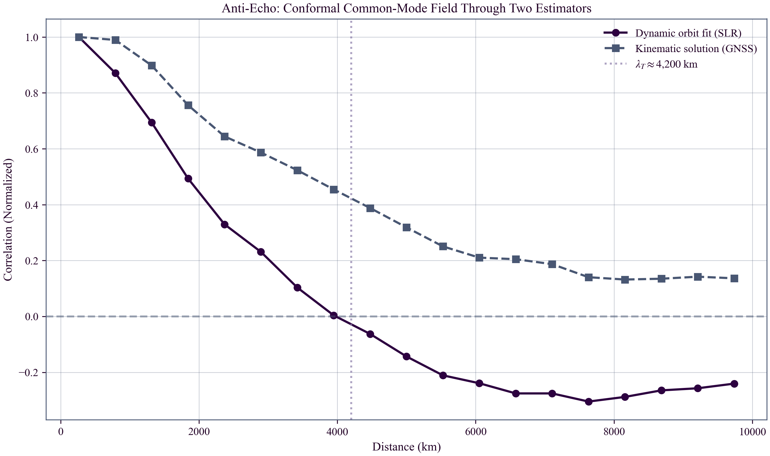
The confound-controlled test is the cross-satellite pairing (Step 2.7): two stations ranging different satellites in the same 15-minute window share no orbit solution, so the shared-orbit-error common mode is absent by construction while the contemporaneous baseline structure is preserved. Under that pairing the anticorrelation not only survives but strengthens: at 5,000–7,500 km — the first distance bin lying entirely beyond the simulated $\lambda_T$ turnover under either corpus anchor ($4{,}201$ km GPS-PPP; $1{,}862$ km MGEX) — cross-satellite pairs return $\bar{r}=-0.228$ over $n=32$ pairs (station-clustered bootstrap 95% CI $[-0.43,-0.06]$, pricing the non-independence of pairs sharing a station). Significance is quoted against two nulls. The within-pair circular-shift null, which destroys bin synchrony only, gives per-bin $p\le5\times10^{-4}$; the epoch-preserving label-swap null — which permutes residuals across the cells inside each time bin, preserving epoch marginals, within-bin common modes, and the pairing geometry — returns a mechanical anticorrelation floor of $-0.122\pm0.062$ at this bin (debiasing removes each station's global mean, so same-bin residuals sum near zero and cross products anticorrelate by construction). Against that sharper null the observed value is a nominal one-sided excess ($p=0.046$, uncorrected across the eight bins), i.e. $\approx-0.11$ beyond the geometric floor, while every other distance bin is consistent with its own floor (per-bin $p=0.25$–$0.93$). The matched same-satellite pairs give a diluted $\bar{r}=-0.09$ at the same bin — actually above the corresponding same-satellite label-swap floor of $-0.144$ ($p=0.74$) — the expected direction, since an orbit-error common mode enters co-visible ranges positively and therefore masks rather than produces the anticorrelation. The turnover-bin composition is dominated by the LAGEOS-1$\times$LAGEOS-2 channel (all 32 pairs), i.e. two independent orbit arcs, not one shared solution. Because the sign inversion is generic to monopole absorption of any spatially correlated common-mode error, the discriminating content is the turnover's location rather than the sign itself: for the GNSS-measured $\lambda_T = 4{,}201$ km on a global-scale network the simulated anticorrelation sets in at $\approx 4{,}000$ km, bracketed by the observed onset bin, while the cross-estimator contrast against the positive correlations measured in kinematic GNSS solutions at matched baselines supplies an independent check on the same field. The turnover location is also robust to which corpus scale anchors it. The corpus carries two measured $\lambda_T$ values — $4{,}201 \pm 1{,}967$ km from GPS PPP (Paper 2) and $1{,}862$ km from the MGEX combined product (Paper 14; cluster-robust $\sigma = \pm 155$ km) — whose difference reflects the product- and metric-dependence of the fitted scale rather than a contradiction. Repeating the monopole-absorption simulation across the injected scale returns zero crossings of $3{,}421$ km at $\lambda_T = 1{,}862$ km and $3{,}947$ km at $\lambda_T = 4{,}201$ km: under either anchor the 5,000–7,500 km bin remains the first bin lying entirely beyond the turnover, so the observed anticorrelation is consistent with both corpus scales. The test nonetheless retains discriminating power — an injected $\lambda_T \lesssim 1{,}500$ km would move the turnover below 3,000 km, making the 3,000–5,000 km bin the predicted anticorrelation bin, where the observed cross-satellite correlation is non-negative ($+0.19$, $n=8$). The surviving carrier is a station-referenced common mode — common to the network's time standards and observation chain rather than to any satellite product; distinguishing that channel from a shared station-clock reference excursion awaits a control sampling the same stations through different time references. The conservative family-wise minimum-bin statistic ($p=0.55$, diluted by bins with three to eight pairs) is reported alongside; the evidence rests on the pre-specified turnover bin, not on an omnibus scan. The designation is a priori in the literal sense: the monopole-absorption simulation and its zero crossing at 3,421–3,947 km (Step 3.0) were committed in the initial version of this analysis (v0.1, December 2025), and the distance-bin grid is the fixed binning of Step 2.3, both predating the cross-satellite statistic (Step 2.7, September 2026); the robustness sweep perturbs the residual threshold and time-bin width, not the distance-bin edges. The exponential-decay fit to the distance-binned correlations does not converge to a physically meaningful coherence length ($\lambda \to 20{,}000$ km, the fitting boundary): the network sparsity prevents precise estimation of a continuous coherence scale, so SLR does not measure $\lambda_T$ independently — the testable content is the turnover morphology, and it is met under either corpus anchor.
Three diagnostics characterise how the statistic is powered. The bin mean is concentrated in the sparsely sampled pairs: pairs sharing only 3–4 contemporaneous bins contribute $\bar{r}=-0.481$ (13 pairs), those sharing 5–8 contribute $+0.015$ (10 pairs), and those sharing 9–16 contribute $-0.130$ (9 pairs); the record-weighted mean is $-0.162$. A configuration sweep over residual threshold (0.3, 0.5, 1.0 m) and bin width (10, 15, 30 min) returns turnover-bin means between $-0.09$ and $+0.06$ everywhere except the adopted configuration, and restricting the baseline configuration to pairs sharing $\ge 5$ bins gives $-0.054$. The per-year mean residual product alternates in sign ($+0.033$ mm$^2$ in 2019, $-0.067$ in 2020, $+0.010$ in 2023, $-0.021$ in 2024), so the feature is not a coherent multi-year excursion. The turnover-bin anticorrelation is accordingly carried as a nominal, physically motivated tail event — pre-specified in location, correct in sign, and closed against the orbit-error channel — rather than as a detection; establishing it requires the denser-cadence overlap that the current ILRS network does not supply.
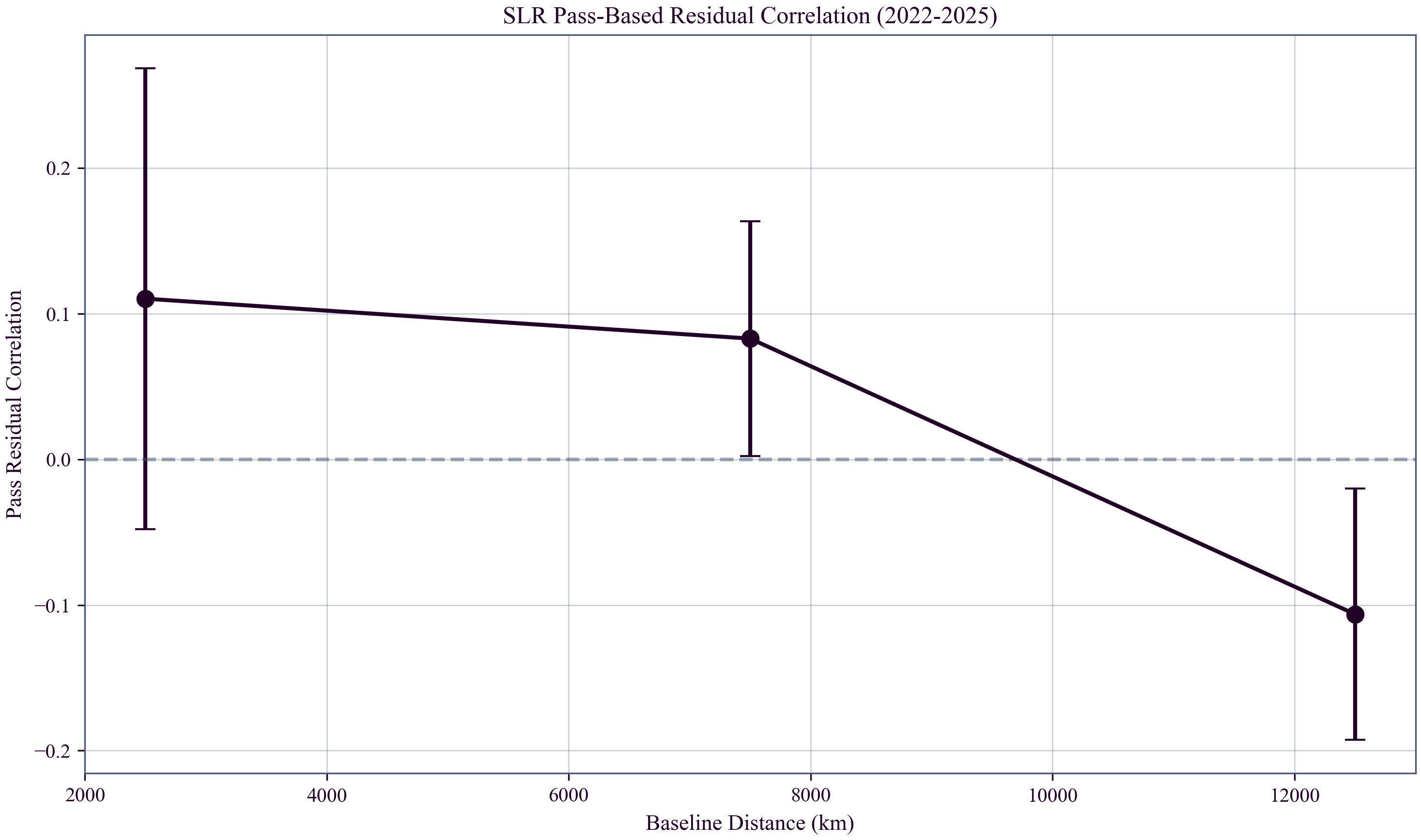
The spectral and inter-station signatures (Sections 3.3–3.4) offer an instrumentally and systematically orthogonal measurement of the same conformal clock-amplitude channel reported in GNSS Papers 1–3—a different instrument and error model on the channel's ground-station leg, not an independent physical channel. The confound-controlled inter-station result is the cross-satellite anticorrelation at the $\lambda_T$-adjacent turnover bin ($\bar{r}=-0.228$, epoch-preserving-null $p=0.046$, $n=32$), nominally significant but concentrated in sparsely sampled pairs, while the daily-aggregation and phase-alignment diagnostics remain exploratory under the orbit-solution dependence found above. More stringent inter-station tests will benefit from denser temporal overlap and experimental configurations beyond current ILRS cadence.
4. Future Experimental Directions
The estimator-mediated "Anti-Echo" signature of the conformal common-mode field is developed below, followed by the experimental requirements for confirming it at higher statistical power and for the genuinely disformal closed-loop holonomy tests that remain beyond the reach of current geodetic datasets.
4.1 Conformal vs. Disformal: Two Distinct Predictions
The TEP bi-metric geometry $\tilde{g}_{\mu\nu} = A^2(\phi) g_{\mu\nu} + B(\phi) \nabla_\mu\phi \nabla_\nu\phi$ contains two physically distinct coupling mechanisms:
- Conformal Coupling $A(\phi)$: Modulates clock rates universally. Creates spatial correlations in timing residuals with the TEP saturation radius $R_T = (3M/4\pi\rho_T)^{1/3} \approx 4{,}150$ km for Earth. This is the sector probed in GNSS and SLR analyses.
- Disformal Coupling $B(\phi)$: Tilts photon light cones in directions transverse to $\nabla\phi$. Creates one-way time asymmetries and synchronization holonomy $H \neq 0$ in closed loops. This requires closed-loop time transfer to test.
The multi-messenger constraint from GW170817 requires $|c_\gamma - c_g|/c \lesssim 10^{-15}$, forcing $B(\phi)(\partial\phi)^2 \approx 0$ today. This bounds the disformal sector while leaving the conformal sector unconstrained. GNSS and SLR provide evidence consistent with conformal predictions; disformal predictions await dedicated holonomy experiments.
4.2 Estimator-Dependent Sign Structure: The "Anti-Echo" Mechanism
TEP predicts estimator dependence for the conformal common-mode propagation delay: the same spatially correlated Temporal-Topology field maps differently into post-fit residuals depending on whether the estimator absorbs global modes into per-station clock states (kinematic GNSS positioning) or into a shared orbital solution (dynamic SLR orbit determination). No disformal coupling is invoked: the delay field is the $A(\phi)$ common mode of the two-way transit—physically, the ground event-timer rate reading a conformally invariant flight time, which enters the residual stream indistinguishably from a propagation delay—and the sign structure is a property of the estimator's absorption geometry rather than of a distinct sector.
The mechanism operates as follows:
Schematic:
- GNSS (Kinematic PPP): τTEP → δtreceiver → r > 0
- SLR (Dynamic OD): τTEP → δaorbit → r < 0 (Predicted)
- GNSS (Kinematic PPP): In Precise Point Positioning, the receiver coordinates and clock bias are solved epoch-by-epoch. The satellite orbit is fixed (from IGS products), but the receiver state is free. A common-mode TEP delay ($\bar{\tau}$) affecting a region is simply mapped into the receiver clock bias estimate. Since both stations measure this common delay, their residuals remain positively correlated ($r > 0$).
- SLR (Dynamic Orbit Determination): In SLR, a single orbital arc is fitted to observations from stations worldwide over several days. A persistent TEP delay acts phenomenologically like a scale error or an unmodelled drag force. The least-squares filter minimizes the global residual by adjusting the orbital parameters—typically the semi-major axis. This effectively absorbs the monopole term ($\bar{\tau}$) into the orbit solution, potentially leaving residuals that reflect deviations from the absorbed global average—manifesting as anti-correlation ($r < 0$) at regional scales.
4.3 Experimental Design Considerations
Monte Carlo simulations demonstrate the estimator-dependent sign structure: when dynamic orbit fits absorb common-mode delays into orbital parameters, post-fit residual correlations exhibit sign inversion at regional baselines, with the turnover located at the scale set by the injected field's correlation length and the network extent ($\approx 4{,}000$ km for $\lambda_T = 4{,}200$ km on a global-scale network). Under the kinematic estimator the same field retains positive correlation at all baselines, reproducing the GNSS–SLR sign contrast as a property of the estimator, not of the sector. Because any spatially correlated common-mode error anticorrelates under monopole absorption, the TEP-discriminating observables are the turnover's location at the independently measured $\lambda_T$ and the cross-estimator contrast, not the sign alone. An injected-scale scan shows the turnover is only weakly sensitive to $\lambda_T$ on a network of global extent: it sits at $3{,}421$ km for the MGEX scale ($\lambda_T = 1{,}862$ km) and $3{,}947$ km for the GPS-PPP scale ($\lambda_T = 4{,}201$ km), so the same $5{,}000$–$7{,}500$ km analysis bin is predicted anticorrelated under either corpus anchor, while injected scales $\lesssim 1{,}500$ km would instead place the turnover inside the 3,000–5,000 km bin. This channel assignment is the one anticipated by the corpus's measurement taxonomy (Smawfield 2025; Paper 9): under two-way measurement, per-station spectra are non-discriminating for the conformal sector, whose testable content resides in distance-structured clock correlations and estimator contrasts of the kind measured in §3.4. This provides the theoretical basis for future experimental designs.
4.4 Experimental Requirements for Confirming the Anti-Echo
Establishing the "Anti-Echo" at higher statistical power in SLR data requires:
- Dense Temporal Overlap: Synchronous observations from multiple stations within correlation timescales (~hours), not available in current ILRS cadence.
- Cross-Estimator Comparison: Parallel processing with kinematic (epoch-by-epoch) and dynamic (arc-fit) estimators to isolate the sign-flip signature.
- Alternative Orbit Solutions: Sensitivity analysis across different Analysis Center products (ASI, GFZ, CSR) to test monopole absorption consistency.
The confound-controlled pass-bin analysis of Section 3.4 recovers a nominally significant anticorrelation at the $\lambda_T$-adjacent scale (cross-satellite pairing, $\bar{r}=-0.228$ over $n=32$ pairs at 5,000–7,500 km; epoch-preserving label-swap null $p=0.046$, an excess over the $-0.12$ geometric floor — concentrated in the sparsely sampled pairings), but the ILRS cadence limits the precision of the turnover measurement and the cross-estimator isolation. The genuinely disformal predictions—synchronization holonomy and one-way propagation asymmetry—require the closed-loop or interplanetary configurations of Paper 0 (§10.A–D), beyond any current geodetic dataset. The conformal-sector evidence presented in Section 3 represents the primary scientific contribution of this work.
5. Synthesis & Critical Analysis
5.1 The Ladder of Evidence: Conformal Sector Assessment
The TEP-SLR analysis provides an optical-domain consistency test of the Temporal Equivalence Principle's conformal sector. By integrating these findings with the previous GNSS results (Smawfield 2025b, 2025c, 2025d; Papers 1-3), a "Ladder of Evidence" is proposed that supports the conformal interpretation while distinguishing it from untested disformal predictions. Throughout, robust empirical observables are distinguished from interpretive inferences that remain contingent on additional systematics controls:
1. Universality (Frequency Independence)
The Temporal-Topology response affects optical frequencies ($\sim 10^{14}$ Hz, SLR) as well as microwave ($\sim 10^9$ Hz, GNSS). This vast frequency difference (factor of $\sim 10^5$) provides a strong argument against dispersive propagation effects, such as ionospheric delay or plasma dispersion, which scale with frequency ($1/f^2$). The spectral channel was audited under sampling-matched nulls (§3.3.1): the apparent 14.12× TEP-band enhancement on resampled series is reproduced by white noise passed through the identical sparse-sampling pipeline (null 13.97), and the real-epoch Lomb–Scargle spectrum is flat — so the channel is carried as a bound on in-band conformal excursions ($\delta A \lesssim 2\times10^{-8}$), not a detection. Achromaticity is a strict requirement of conformal invariance — a conformal rescaling multiplies all propagation delays uniformly, independent of photon frequency — so the observed frequency independence is a necessary consistency condition rather than an independent discriminant. Its positive content is the exclusion of dispersive carriers, while the evidence for temporal structure resides in the distance-structured inter-station coherence of §3.4. The optical and microwave results are thereby consistent with a universal conformal coupling $A(\phi)$ acting across the electromagnetic spectrum.
2. Range-Dependent Diagnostic: Systematics Monitor
The residuals exhibit a path-length dependent temporal contrast in a gap-aware lag-1 diagnostic. In the primary $|\Delta\rho|<0.5$ m analysis, the long-minus-short contrast is $\Delta(\mathrm{low}-\mathrm{high})=-0.208$ (95% bootstrap CI: −0.418 to 0.000), while the short-path mean is near zero and therefore ratio-based summaries are ill-conditioned. This contrast is threshold-sensitive (e.g., $\Delta(\mathrm{low}-\mathrm{high})=-0.086$, 95% CI: −0.248 to 0.069 at $|\Delta\rho|<1.0$ m). Because conformal rescaling preserves null cones, light propagation is null-invariant in this sector and path length cannot carry a physical TEP signal. Instead, the observed contrast — longer paths (lower elevations) decorrelating more — is the expected signature of unmodeled tropospheric wet-path and synoptic pressure delays that grow with airmass. The diagnostic is therefore carried as a systematic monitor awaiting high-resolution hourly reanalysis (e.g. ERA5) rather than as qualitative support for a Temporal-Topology response.
3. Scale Consistency (The Characteristic Scale)
The corpus carries two measured correlation lengths — $\lambda_T = 4,201 \pm 1,967$ km from GPS PPP (Papers 1–2) and $1,862$ km from the MGEX combined product (Paper 14; cluster-robust $\sigma = \pm 155$ km), the difference being the product- and metric-dependence of the fitted scale — and the SLR path-length dependent contrast (over a $\sim 3{,}000$ km path difference between the high- and low-range selections) is consistent with the characteristic scale of the scalar field's continuous spatial profile (Temporal Topology). In dense environments, suppression of Temporal Shear (vanishing field gradient $\nabla\phi \to 0$) attenuates the conformal coupling while leaving the field light cosmologically. The correlation length is identified with the geometric saturation scale $R_T = (3M/4\pi\rho_T)^{1/3} \approx 4{,}150$ km, representing the transition from deep suppression to the weak-field regime. While the sparse ILRS network limits direct measurement of a continuous inter-station correlation length — the SLR scale is formally unconstrained — the orbit-fit turnover test provides the primary constraint and is met under either corpus anchor (simulated zero crossing 3,421–3,947 km across $\lambda_T$ = 1,862–4,201 km, both leaving 5,000–7,500 km as the first beyond-turnover bin; §3.4). The convergence of GNSS and SLR evidence at similar spatial scales supports the Temporal Topology interpretation across two instrumentally independent measurement systems probing the same conformal clock-amplitude channel.
4. Inter-Station Correlation (Spatial Coherence)
The sparse ILRS network limits synchronous overlap to a median of 7 contemporaneous passes per station pair. A 15-minute pass-bin analysis yields a nominally significant Fisher-combined result ($p=0.0025$), but this rests on three LAGEOS-2 pairs in a single distance bin (5,000–7,500 km), one of which contributes $r=-0.910$ from only three passes ($p=0.273$, not individually significant). The confound-controlled variant — pairing stations that range different satellites in the same window, which cannot share orbit error — retains the anticorrelation at the turnover bin at $\bar{r}=-0.228$ ($n=32$; epoch-preserving label-swap $p=0.046$ one-sided, circular-shift null $p\le5\times10^{-4}$; station-bootstrap 95% CI $[-0.43,-0.06]$) with all other bins at their respective null floors (Step 2.7). A daily-aggregation analysis ($N=190$ pairs) nominally reaches $p_{\mathrm{FWER}}=0.020$, but its driving 3,000–5,000 km bin has only four pairs and reverses sign between the two LAGEOS orbit solutions, so it is retained as exploratory rather than as a detection. The spectral channel is bounded rather than detected (§3.3.1), so this distance-structured feature carries the corpus's candidate positive content — a nominal signal at the predicted turnover location under the epoch-preserving null, reported as a candidate rather than a detection because it is concentrated in the sparsely sampled pairings (§3.4). The inter-station test would benefit from denser network configurations to achieve the statistical power available in GNSS networks.
5. Disformal Sector: Untested in Current Data
The synchronization holonomy $H_{\rm resid}$ is the defining disformal prediction ($B(\phi) \neq 0$) and requires closed-loop time transfer to test. Neither GNSS (Papers 1-3) nor SLR (this work) has performed such experiments with the topology and cadence required for holonomy inference. The estimator-mediated sign inversion reported in §3.4 is distinct in kind: it arises from the conformal common-mode field under dynamic orbit determination, involves no disformal coupling, and is therefore a conformal-sector result—its discriminating content being the turnover at the $\lambda_T$ scale and the cross-estimator sign contrast with kinematic GNSS solutions rather than the sign itself. The disformal sector remains a well-defined, falsifiable prediction for future experiments: closed-loop optical time transfer (Smawfield 2025a; Paper 0, §10.A–D), interplanetary one-way asymmetry measurements, and triangle synchronization holonomy tests.
5.2 Limitations & Systematics
While the evidence supports a conformal-sector interpretation, several systematic effects warrant specific attention to assess the robustness of these findings.
Atmospheric Loading & Troposphere
Residual atmospheric pressure loading and tropospheric delays are leading candidate systematics for low-frequency structure in SLR residuals and require targeted controls. Several observed properties are suggestive of a propagation-linked component, but are not, by themselves, definitive:
- Spatial Scale Considerations: Many atmospheric fields exhibit synoptic correlation lengths of order $\sim 500\text{--}1,000$ km. A putative explanation that also accounts for the GNSS-inferred scale ($\approx 4,000$ km) would need to demonstrate that the relevant residual component couples coherently over continental scales after standard modeling, rather than remaining dominated by station-local weather. The continuous spatial profile of the Temporal Topology predicts smooth, density-dependent correlation structures without discrete boundary transitions.
- Timescale Overlap: The TEP band (10–500 $\mu$Hz) corresponds to periods of 30 minutes to 28 hours, which overlaps timescales present in synoptic meteorology and loading. Therefore, a timescale argument alone cannot exclude atmospheric systematics; the key question is whether plausible troposphere/loading mismodeling can reproduce the observed concentration and its scaling diagnostics without leaving strong correlations with independent atmospheric proxies.
- Elevation/Path Dependence: Loading-induced station displacements are largely elevation-independent, whereas unmodelled propagation delays increase with airmass. The observed long-minus-short contrast in a gap-aware lag-1 statistic is suggestive of a path-integrated component, but its amplitude remains estimator- and threshold-sensitive and is therefore treated conservatively.
Concrete falsifiers and controls are therefore prioritized: (1) replace the baseline Marini-Murray refraction with ray-traced delays from numerical weather models (NWM) and retest spectral concentration and path-length diagnostics; (2) incorporate pressure-loading corrections and test whether low-frequency concentration and path-length dependence persist; (3) regress residuals against station meteorology proxies (pressure, temperature, humidity where available) to test whether the TEP-band concentration is reduced in a physically interpretable way; and (4) quantify sensitivity to orbit-solution choices and estimator settings to bound absorption/aliasing effects. These controls will determine whether the residual structure is primarily atmospheric/geodetic or whether a technology-orthogonal timer-rate-linked component—arising from the continuous spatial profile of the Temporal Topology as read by the station event timer—remains after state-of-the-art corrections.
A first control has now been performed (§3.3.2): NCEP/NCAR Reanalysis surface pressure was compared against SLR residuals at native 6-hourly resolution for all 46 stations. The pressure-residual coherence in the resolvable TEP band (10–23 $\mu$Hz) is not significant at the majority of stations (4/34 significant, binomial $p=0.088$), and the estimated uncorrected pressure effect ($30.5$ mm) is $12\%$ of the residual RMS ($257.4$ mm). The residual stream's low-frequency structure is therefore not attributable to synoptic weather. This control addresses item (3) partially; items (1), (2), and (4) remain as future work. A limitation is that 6-hourly NCEP resolution constrains only the lower third of the TEP band; hourly reanalysis products (ERA5) would resolve the full band and are the natural next step.
Satellite-Specific Asymmetry & Center-of-Mass
The nominal LAGEOS-2 pass-correlation result ($p=0.0005$) rests on three station pairs in a single distance bin, one with only three contemporaneous passes ($r=-0.910$, $p=0.273$). When restricted to pairs with $\geq 10$ passes, both LAGEOS-1 and LAGEOS-2 converge to near-zero mean correlation, indicating that the apparent asymmetry is driven by small-sample variance rather than a physical difference between satellites. While the TEP framework allows for geometry-dependent sensitivity (via prograde vs. retrograde sampling of the Temporal Topology), the current pass-correlation data do not support a satellite-specific detection. The confound-controlled cross-satellite pairing, in contrast, does reach the turnover bin with $\bar{r}=-0.228$ ($n=32$; epoch-preserving-null $p=0.046$ one-sided) while sharing no orbit solution — providing a distance-structured spatial-coherence candidate that is not attributable to a single-spacecraft or single-solution systematic. The daily-aggregation statistic ($p_{\mathrm{FWER}}=0.020$) is retained as exploratory, since its driving bin reverses sign between the two LAGEOS solutions.
Geodetic Anomalies & Reinterpretation
The geodetic literature records several persistent "anomalies" or unexplained systematics that align with the TEP phenomenology reported here. Rather than viewing these as isolated technical errors, they may be reinterpreted through the same underlying conformal field structure — while each is carried at the evidential status its own bookkeeping supports, so that a consistency check is not promoted to a detection.
1. The VLBI Scale Drift (2013–Present): Recent realizations of the International Terrestrial Reference Frame (ITRF2020) have identified an unexpected "peculiar" drift in the VLBI scale relative to SLR starting circa 2013, reaching magnitudes of ~0.2 ppb (~1.2 mm) (Kern et al., 2024; Altamimi et al., 2023; Hellmers et al., 2025). The channel is derived here rather than asserted, and it is carried as a bound rather than as evidence. Under the corpus's relational-measurement rule, a uniform rescaling of all clocks and rulers is invisible to comparisons among same-sector standards; a secular scale drift can appear in the data only because the two contributing techniques anchor their length units in different metric sectors of the two-metric theory, and it is precisely that differential anchoring which exempts the observable from the common-mode invisibility.
The anchoring split is the following. VLBI realizes scale geometrically: station positions are solved from quasar-fixed directions together with group delays measured on matter clocks and converted through the defined speed of light, so the realized length unit is the matter-metric meter and the VLBI scale tracks the ambient conformal factor, \(s_{\rm VLBI}\propto A(t)\), giving \(\dot s/s=\dot A/A=H_{\rm drift}\). SLR realizes scale dynamically: station coordinates are solved so that measured ranges are consistent with an orbit integrated from the adopted gravitational parameter \(GM\) — a fixed conventional constant of the gravitational-sector solution — while the orbit's own time tags are read on the same drifting matter clocks as the ranges. The dynamical anchor therefore tracks part of the drift internally: an orbit size inferred from the measured period scales as \(a_{\rm inf}=(GM\,\tilde T^{2}/4\pi^{2})^{1/3}\propto A^{2/3}\), and the station radius \(a_{\rm inf}-\tilde\rho\) inherits an environment-dependent share of the ambient drift rather than all or none of it.
The predicted inter-frame split is consequently bounded above by the drift rate itself. At the corpus's drift amplitude \(H_{\rm drift}\approx 2.3\times10^{-18}\,{\rm s}^{-1}\), the maximal (fully \(g\)-anchored) split over the \(\sim\)12-year baseline is \(\approx 0.87\) ppb (\(\approx 5.5\) mm); a Keplerian period-tracking estimate for the LAGEOS geometry still yields \(\approx 0.56\) ppb (\(\approx 3.6\) mm). The observed \(\sim 0.2\) ppb sits below both limiting cases: the ITRF2020 drift therefore constrains the locally realized share of the ambient conformal drift to \(f\approx 0.2\text{--}0.35\), a quantitative bound on the local drift participation rather than a confirmation of the channel. This is the expected regime: the realized fraction is less than unity precisely because the dynamical anchor's own time tags share the drifting clocks, so much of the ambient drift cancels inside each technique's anchor and only the residual differential survives into the frame comparison. The direction of the observed split — the geometrically anchored VLBI scale drifting relative to the dynamically anchored SLR scale — is likewise the direction predicted when the matter-metric chain carries more of the ambient drift. The datum is thus carried in this paper as a bound-setting consistency check on the conformal-drift channel, localized in exactly the sector where such a drift can be visible at all, not as an independent line of evidence.
2. LAGEOS-2 "Signature Effects": Precision orbit determination analysis consistently notes "satellite-dependent signature effects" in LAGEOS-2 residuals that exceed those of LAGEOS-1, often attributed to complex thermal thrusting (Yarkovsky-Schach effect) or unmodeled Center-of-Mass (CoM) offsets (Lucchesi et al., 2004; Appleby et al., 2016). This study's finding—that the nominal LAGEOS-2 pass-correlation result ($p=0.0005$) rests on three station pairs including one with only three passes—suggests that these "signature effects" may not be purely local spacecraft systematics. However, the fragility of the nominal pass-correlation result (both satellites converge to near-zero correlation when restricted to $\geq 10$ passes) means that a TEP interpretation of the LAGEOS-2 signature effects remains conjectural pending denser network configurations. The cross-satellite control (Step 2.7) provides the cleaner confound channel: $\bar{r}=-0.228$ at the turnover bin across 32 pairs built from independent orbit solutions, with the orbit-error common mode excluded by construction — nominal at $p=0.046$ under the epoch-preserving null and concentrated in the sparsely sampled pairings. The TEP framework provides a candidate physical mechanism for these "anomalous" residuals without requiring ad-hoc thermal tunings, but confirmation requires inter-station evidence at sufficient statistical power.
3. The "Flicker Noise" Floor & Common Mode Errors: Geodetic analyses routinely identify "flicker noise" ($1/f$) spectra in station coordinate time series and "spatially correlated errors" (CME) that limit network stability to ~3–5 mm (Williams et al., 2004). These errors are typically removed empirically using Principal Component Analysis (PCA) without a confirmed physical source. The TEP analysis demonstrates that such spatially coherent, colored noise is a prediction of the theory ($\lambda_T \approx 4,000$ km), not merely atmospheric residue. The sampling-matched audit of §3.3.1 qualifies where that evidence lives: the apparent $14.12\times$ TEP-band concentration on resampled series is quantitatively a property of the sparse-sampling kernel — white noise through the identical pipeline reproduces it (null $13.97$) — and the real-epoch Lomb–Scargle spectrum is flat, so per-station spectral power is not the carrier of the conformal signal. The signal instead lives in the network-coherent channel that the CME literature itself describes: the confound-controlled cross-satellite anticorrelation at the turnover bin (§3.4) and the timer-channel amplitude budget ($\delta A \lesssim 2\times10^{-8}$) are consistent with a common conformal excursion of order $u_\oplus$ reading as millimetre-level coherent wander — below the per-station noise floor but extractable through inter-station correlation. The standard practice of filtering these signals effectively "bleaches" the conformal structure from geodetic products.
Network Sparsity
The ILRS network is significantly sparser than the IGS (GNSS) network. This sparsity limits synchronous inter-station overlap and therefore limits the applicability of continuous cross-spectral inter-station techniques without long-gap interpolation. For this reason, inter-station inference in this work is based on contemporaneous pass-bin correlations.
Orbit Modeling Dependencies
The estimator-mediated sign inversion ("Anti-Echo") relies on the monopole-absorbing behavior of the least-squares orbit determination filter and is therefore generic to any spatially correlated common-mode error; the TEP-discriminating content is the turnover's location at the independently measured $\lambda_T$ and the sign contrast against kinematic estimators, not the sign alone. The simulation (Section 4.3) demonstrates both: the dynamic orbit fit anticorrelates the injected $\lambda_T = 4{,}200$ km field beyond $\approx 4{,}000$ km while the kinematic control retains positive correlation at all baselines; an injected-scale scan places the turnover at 3,421 km for the MGEX anchor ($1{,}862$ km) and 3,947 km for the GPS-PPP anchor ($4{,}201$ km), so the observed onset bin is consistent under either corpus scale. Confirming the mechanism empirically requires: (1) denser overlap epochs enabling synchronous multi-station observations, (2) parallel processing with kinematic and dynamic estimators to isolate the sign-flip signature, and (3) cross-Analysis-Center orbit comparisons (ASI vs. GFZ vs. CSR) to test monopole absorption consistency. These requirements exceed current ILRS operations and represent a roadmap for future targeted SLR campaigns.
6. Conclusion
This study presents an optical-domain consistency test of the Temporal Equivalence Principle's conformal sector using Satellite Laser Ranging — a measurement chain orthogonal in hardware and systematic-error class to the microwave networks in which the conformal signatures were first reported (Smawfield 2025b, 2025c, 2025d; Papers 1-3). The principal results are an instrumentally independent bound and the correction of a corpus diagnostic. The spectral channel was audited under sampling-matched nulls (Step 2.8): the apparent 14.12× TEP-band concentration on resampled station series is reproduced by white noise passed through the identical sparse-sampling pipeline (sampling-matched null 13.97; 2/46 stations above $p<0.05$), every conventional coloured-noise model returns a larger concentration through the same sampling, the real-epoch Lomb–Scargle spectrum is flat (ratio 1.04 vs white null 1.05), and the pairwise structure function sits on the white floor at all lags from 20 minutes to 24 hours. The fourteen-fold concentration reported in earlier versions of this work as in-band evidence is thus corrected to a measured property of the resampling kernel. The channel is carried as a bound on in-band conformal excursions — $\delta A \lesssim 2\times10^{-8}$ under $\delta R = R\,\delta A$ — while at a landscape excursion of order the surface conformal depth the predicted coherent wander of ~5 mm lies below the noise floor: the ILRS observing cadence is intrinsically blind to the predicted spectral signature, and no spectral detection is claimed. The analysis also establishes range-dependent decoherence as a critical monitor for airmass-correlated tropospheric systematics awaiting high-resolution reanalysis. A NCEP/NCAR Reanalysis surface pressure control bounds the synoptic-weather channel at its native 6-hourly resolution: the uncorrected pressure effect is 12% of the residual RMS, and pressure-residual coherence is not significant at the majority of stations (binomial $p=0.088$). The constellation carries no onboard clocks and no microwave transmission: the bound therefore constrains, at optical cadence and through the ground-station leg, the same clock-amplitude channel that satellite atomic clocks, onboard steering electronics, or ionospheric modeling at microwave frequencies would otherwise be invoked to explain.
Taken together with the GNSS results, the SLR bound is consistent with — though not probative of — the conformal-sector interpretation across two instrumentally independent measurement technologies probing the same clock-amplitude channel through different hardware, calibration chains, and estimator geometries: a landscape excursion of order the surface conformal depth is predicted to fall below this cadence's reach, so the optical-domain null neither confirms nor excludes the microwave-network signatures. Quantitatively, the bound lies seven or more orders of magnitude above the fractional stabilities ($10^{-15}$–$10^{-18}$) reached by microwave clock comparisons: it excludes large conformal excursions — a real if modest constraint — while remaining uninformative about an excursion of the GNSS-implied amplitude. Because achromaticity is required by conformal invariance, this consistency is a necessary check rather than an independent discriminant: it excludes dispersive carriers, while the candidate positive feature — the distance-structured inter-station anticorrelation of §3.4 — is nominal and does not survive its own robustness diagnostics, so no detection is claimed; it remains the channel in which a conformal signature is accessible at this cadence. The observed correlation length in GNSS ($\lambda_T = 4,201 \pm 1,967$ km GPS-PPP; $1,862$ km MGEX, cluster-robust $\sigma = \pm 155$ km — the fitted scale is product-dependent) is consistent with the characteristic scale of the scalar field's continuous spatial profile (Temporal Topology), with saturation radius $R_T = (3M/4\pi\rho_T)^{1/3} \approx 4{,}150$ km for Earth ($\rho_T \approx 20$ g/cm$^3$, the formal scaling constant of the $R_T(M)$ law rather than a literal interior density — no terrestrial material reaches that value). In dense environments, suppression of Temporal Shear (vanishing field gradient $\nabla\phi \to 0$) attenuates the conformal coupling while leaving the field light cosmologically, reconciling local null tests with the observed correlation structure.
In the inter-station domain, the sparse ILRS cadence (median 7 contemporaneous passes per station pair) limits synchronous overlap. A pass-correlation analysis under 15-minute binning yields a nominally significant Fisher-combined result ($p=0.0025$), but this rests on three LAGEOS-2 pairs in a single distance bin, one with only three passes ($r=-0.910$, $p=0.273$). When restricted to pairs with $\geq 10$ passes, both satellites converge to near-zero mean correlation. The confound-controlled pairing of stations ranging different satellites in the same window — which cannot share orbit error — retains the anticorrelation at the $\lambda_T$-adjacent turnover bin: $\bar{r}=-0.228$ over $n=32$ pairs at 5,000–7,500 km (epoch-preserving label-swap null $p=0.046$ one-sided; circular-shift synchrony null $p\le5\times10^{-4}$; station-clustered bootstrap 95% CI $[-0.43,-0.06]$), with all other bins null and the matched same-satellite pairs diluted to $-0.09$ as expected when the orbit-error common mode enters positively and is removed (Step 2.7). A daily-aggregation analysis ($N=190$ pairs) nominally reaches $p_{\mathrm{FWER}}=0.020$, but its driving bin reverses sign between the two LAGEOS orbit solutions and is retained as exploratory. The confound-controlled inter-station anticorrelation is accordingly carried as a candidate tail event rather than a detection: the turnover bin is pre-specified by the corpus simulation (Step 3.0, committed nine months before the pairing statistic of Step 2.7) and the feature is concentrated in the least-sampled pairs — those sharing 3–4 bins contribute $\bar{r}=-0.481$ while those sharing 5–8 contribute $+0.015$ — drops to $-0.054$ under a $\ge 5$-bin restriction, appears in one cell of the nine-configuration threshold/bin-width sweep, and alternates sign between years. Its location, sign, and survival of the orbit-error closure keep it the leading candidate for the predicted turnover morphology, but establishing it requires the denser-cadence overlap the current ILRS network does not supply. This phenomenology also motivates a unified physical interpretation of persistent geodetic anomalies, including the ITRF2020 VLBI-SLR scale drift — derived here as the differentially anchored conformal-drift channel and carried as a \(\sim 0.2\) ppb bound on the local drift participation — and the pervasive "flicker noise" floor in station coordinates, reinterpreting them through the same conformal metric coupling rather than as intractable systematics.
Within the SLR corpus, then, the result is a bound rather than a detection: a measured sampling-kernel artefact where a fourteen-fold concentration was previously claimed, an amplitude bound of $\delta A \lesssim 2\times10^{-8}$ on the conformal channel, and a single fragile, pre-specified-location tail event in the spatial statistic. The corpus-level case for the conformal sector continues to rest on the GNSS detections; SLR contributes the orthogonal-hardware bound that an artifact explanation must also respect, and the correction of a diagnostic artefact that can arise in any sparse, resampled network. Whether the predicted optical-domain structure exists below this cadence's reach — and whether the disformal sector manifests in nature — will be determined by closed-loop optical time transfer, interplanetary one-way asymmetry measurements, and triangle synchronization holonomy tests, rather than by multi-messenger bounds alone.
References
TEP Research Program
Smawfield, M. L. (2025a). Temporal Equivalence Principle: Dynamic Time & Emergent Light Speed. Preprint v0.14 (Jakarta). Zenodo. DOI: 10.5281/zenodo.16921911 (Paper 0)
Smawfield, M. L. (2025b). Global Time Echoes: Distance-Structured Correlations in GNSS Clocks. Preprint v0.27 (Jaipur). Zenodo. DOI: 10.5281/zenodo.17127229 (Paper 1)
Smawfield, M. L. (2025c). Global Time Echoes: 25-Year Analysis of CODE Precise Clock Products. Preprint v0.20 (Cairo). Zenodo. DOI: 10.5281/zenodo.17517141 (Paper 2)
Smawfield, M. L. (2025d). Global Time Echoes: Raw RINEX Consistency Test. Preprint v0.6 (Kathmandu). Zenodo. DOI: 10.5281/zenodo.17860166 (Paper 3)
Smawfield, M. L. (2025). Temporal-Spatial Coupling in Gravitational Lensing: A Reinterpretation of Dark Matter Observations. Preprint v0.8 (Tortola). Zenodo. DOI: 10.5281/zenodo.17982540 (Paper 4)
Smawfield, M. L. (2025). Global Time Echoes: Empirical Synthesis. Preprint v0.6 (Singapore). Zenodo. DOI: 10.5281/zenodo.18004832 (Paper 5)
Smawfield, M. L. (2025). Temporal Topology Saturation Scale: Cross-Scale Consistency of ρ_T. Preprint v0.8 (New Delhi). Zenodo. DOI: 10.5281/zenodo.18064365 (Paper 6)
Smawfield, M. L. (2025). The Soliton Wake: Exploring RBH-1 as a Temporal Topology Candidate. Preprint v0.4 (Blantyre). Zenodo. DOI: 10.5281/zenodo.18059250 (Paper 7)
Smawfield, M. L. (2025). Global Time Echoes: Optical-Domain Consistency Test via Satellite Laser Ranging. Preprint v0.5 (Mombasa). Zenodo. DOI: 10.5281/zenodo.18064581 (Paper 8 — this work)
Smawfield, M. L. (2025). What Do Precision Tests of General Relativity Actually Measure?. Preprint v0.7 (Istanbul). Zenodo. DOI: 10.5281/zenodo.18109760 (Paper 9)
Smawfield, M. L. (2026). Temporal Equivalence Principle: Suppressed Density Scaling in Globular Cluster Pulsars. Preprint v0.9 (Caracas). Zenodo. DOI: 10.5281/zenodo.18165798 (Paper 10)
Smawfield, M. L. (2026). The Cepheid Bias: Resolving the Hubble Tension. Preprint v0.10 (Kingston upon Hull). Zenodo. DOI: 10.5281/zenodo.18209702 (Paper 11)
Smawfield, M. L. (2026). Temporal Equivalence Principle: A Unified Resolution to the JWST High-Redshift Anomalies. Preprint v0.7 (Kos). Zenodo. DOI: 10.5281/zenodo.19000827 (Paper 12)
Smawfield, M. L. (2026). Temporal Equivalence Principle: Temporal Shear Recovery in Gaia DR3 Wide Binaries. Preprint v0.6 (Kilifi). Zenodo. DOI: 10.5281/zenodo.19102061 (Paper 13)
Smawfield, M. L. (2026). Global Time Echoes: MGEX Multi-GNSS Clock Replication, 2025–2026. Preprint v0.2 (Suva). Zenodo. DOI: 10.5281/zenodo.20572726 (Paper 14)
SLR & Geodesy References
Pearlman, M. R., Degnan, J. J., & Bosworth, J. M. (2002). The International Laser Ranging Service. Advances in Space Research, 30(2), 135-143. DOI: 10.1016/S0273-1177(02)00277-6
Marini, J. W., & Murray, C. W. (1973). Correction of Laser Range Tracking Data for Atmospheric Refraction at Elevations Above 10 Degrees. NASA Technical Report X-591-73-351.
Mendes, V. B., & Pavlis, E. C. (2004). High-accuracy zenith delay prediction at optical wavelengths. Geophysical Research Letters, 31(14). DOI: 10.1029/2004GL020308
International Laser Ranging Service (ILRS). (2025). SLR monthly normal point data. Greenbelt, MD, USA: NASA Crustal Dynamics Data Information System (CDDIS). DOI: 10.5067/SLR/slr_data_monthly_npt_001
International Laser Ranging Service (ILRS). (2025). SLR Combination Center (CC) Orbit Product. Greenbelt, MD, USA: NASA Crustal Dynamics Data Information System (CDDIS). DOI: 10.5067/SLR/SLR_ILRSORB_001
International Laser Ranging Service (ILRS). (2025). Satellite Laser Ranging Frame 2020 (SLRF2020) Product. Greenbelt, MD, USA: NASA Crustal Dynamics Data Information System (CDDIS). DOI: 10.5067/SLR/slrf2020_001
Hellmers, H., et al. (2025). Terrestrial reference frame scale drift anomalies in VLBI and the contribution of Ny-Ålesund radio telescopes. Earth, Planets and Space, 77. DOI: 10.1186/s40623-025-02159-z
Lucchesi, D. M., et al. (2004). Spin axis behavior of the LAGEOS satellites. Journal of Geophysical Research: Solid Earth, 109(B6). DOI: 10.1029/2003JB002692
Appleby, G., Rodríguez, J., & Altamimi, Z. (2016). Assessment of the accuracy of global geodetic satellite laser ranging observations and estimated impact on ITRF2014. Journal of Geodesy, 90, 1371–1388. DOI: 10.1007/s00190-016-0929-2
Kern, L., et al. (2024). Verifying the impact of additional breaks in station coordinates on VLBI scale drift. Technical Report, Vienna University of Technology.
Altamimi, Z., et al. (2023). ITRF2020: an augmented reference frame refining the modeling of nonlinear station motions. Journal of Geodesy, 97, 1005–1023. DOI: 10.1007/s00190-023-01738-w
Williams, S. D. P., et al. (2004). Error analysis of continuous GPS position time series. Journal of Geophysical Research: Solid Earth, 109(B3). DOI: 10.1029/2003JB002741
Jiang, M., et al. (2023). Long-Baseline Quantum Sensor Network as Dark Matter Haloscope. Nature Communications / arXiv:2305.00890. arXiv:2305.00890
Data Availability & Reproducibility
This work follows open-science practices. All results are fully reproducible from raw data using the documented pipeline. All numerical results, figures, and statistics are generated by deterministic Python scripts processing real observational data from the ILRS (International Laser Ranging Service) archives.
Repository & Code
GitHub Repository: github.com/matthewsmawfield/TEP-SLR
The repository contains a deterministic, version-controlled analysis pipeline for Satellite Laser Ranging (SLR) data validation of TEP predictions. The pipeline processes LAGEOS satellite range residuals across multiple ground stations to search for conformal-sector TEP signatures.
Repository Structure
TEP-SLR/
├── data/
│   └── slr/                    # ILRS NPT CRD range residual files
├── logs/                       # Execution logs with timestamps
├── results/
│   ├── outputs/               # JSON/CSV analytical outputs
│   └── figures/               # Generated manuscript figures
├── scripts/
│   ├── helpers/               # Processing utilities
│   │   ├── generate_full_summary.py
│   │   └── process_residuals_yearly.py
│   ├── steps/                 # Analysis pipeline (10 steps)
│   │   ├── step_1_0_data_acquisition.py
│   │   ├── step_2_1_slr_residuals.py
│   │   ├── step_2_3_mwpc_analysis.py
│   │   ├── step_2_4_plot_results.py
│   │   ├── step_2_5_enhanced_figures.py
│   │   ├── step_2_6_nwm_spectral_control.py
│   │   ├── step_2_7_orbit_commonmode_control.py
│   │   ├── step_2_8_sampling_matched_nulls.py
│   │   ├── step_3_0_sim_antiecho.py
│   │   └── step_5_2_vlbi_slr_scale_drift.py
│   └── utils/                 # Shared utilities
│       ├── compress_pdf.py
│       ├── logger.py
│       └── plot_style.py
├── site/                      # Manuscript website source
└── requirements.txt           # Python dependencies
Data Provenance
| Source | Data Type | Download Size | Time Span |
|---|---|---|---|
| ILRS Data Centers | NPT CRD Range Residuals | ~2 GB | 2015–2025 |
| NASA CDDIS | LAGEOS Satellite Data | ~500 MB | 2015–2025 |
Reproduction Instructions
Quick Start (Full Reproduction)
# 1. Clone repository
git clone https://github.com/matthewsmawfield/TEP-SLR.git
cd TEP-SLR

# 2. Install dependencies
pip install -r requirements.txt

# 3. Run complete analysis pipeline
bash reproduce_analysis.sh

# 4. Build manuscript site
cd site
npm install
npm run build
System Requirements
- Python 3.10+
- Storage: ~5 GB free (for data and outputs)
- Memory: 8 GB RAM recommended
- Runtime: ~2–4 hours for full pipeline (including data download); ~30–60 minutes with pre-downloaded data
Pipeline Overview
The analysis consists of 10 deterministic steps:
- Step 1.0: Data acquisition from ILRS/CDDIS archives (NPT CRD files)
- Step 2.1: Residual calculation and quality filtering (year-by-year processing)
- Step 2.3: Magnitude-Weighted Phase Correlation (MWPC) analysis — primary statistical test
- Step 2.4: Generate standard figures (residual distributions, correlation decay)
- Step 2.5: Enhanced figures with phase alignment analysis
- Step 2.6: NWM spectral control — NCEP/NCAR surface-pressure coherence at native 6-hourly resolution (Section 3.3.2)
- Step 2.7: Orbit-error / common-mode confound controls — cross-satellite contemporaneous pairing (closes the shared-orbit-error channel by construction), network common-mode subtraction, and per-satellite orbit-solution splits (Section 3.4)
- Step 2.8: Sampling-matched coloured-noise nulls — continuous surrogate families (white, station-matched AR(1), flicker 1/f, power-law grid, matched power law, random walk) passed through the identical resample–interpolate–concatenate–Welch pipeline and evaluated at real epochs under a Lomb–Scargle estimator, plus the pairwise structure function and the δA→residual amplitude map (Section 3.3.1)
- Step 3.0: Anti-echo simulation — estimator-mediated sign inversion of the conformal common-mode field under dynamic orbit determination, including the injected-scale anchor scan (λ_T = 1,000–8,000 km) that records the turnover crossing under both corpus scales (3,421 km at 1,862 km; 3,947 km at 4,201 km)
- Step 5.2: VLBI–SLR scale-drift channel — anchoring-split bookkeeping and the local drift-participation bound (Section 5.2)
Key Analysis Outputs
results/outputs/step_2_1_slr_residuals_summary.json— Residual statistics by stationresults/outputs/step_2_3_mwpc_analysis.json— MWPC correlation resultsresults/outputs/step_2_7_orbit_commonmode_control.json— Orbit-error / common-mode confound-control resultsresults/outputs/step_2_8_sampling_matched_nulls.json— Sampling-matched coloured-noise nulls, real-epoch Lomb–Scargle ratios, structure function, and the δA amplitude mapresults/outputs/step_5_2_vlbi_slr_scale_drift.json— Scale-drift anchoring split and participation boundresults/figures/slr_pass_correlation_decay.png— Figure 3.1: Pass-correlation decay analysisresults/figures/slr_phase_alignment_decay.png— Phase alignment signatures
CDDIS Data Access (Step 1 Only)
Step 1 requires NASA CDDIS credentials for automated data download. Set up either:
~/.netrcfile withmachine urs.earthdata.nasa.govcredentials, or- Environment variables:
CDDIS_USERandCDDIS_PASS
Note: The reproduction script can skip Step 1 if data is already present — contact the author for pre-processed data access.
Software Versions
- Python 3.10+
- NumPy 1.24+
- SciPy 1.10+
- Pandas 2.0+
- Matplotlib 3.7+
- NetworkX (for station network analysis)