
Abstract
This paper validates that distance-structured correlations in GNSS clocks exist in raw observations using broadcast ephemerides, not just precise products—strongly constraining precise-product processing artifacts. Broadcast ephemerides still contain control-segment information, so Satellite Laser Ranging and non-GNSS optical checks remain necessary for definitive confirmation. Prior TEP analyses relied on precise orbit and clock products from global analysis centers, leaving open the possibility that observed signatures were artifacts of sophisticated processing chains. This paper addresses that concern by detecting distance-structured signatures in raw GNSS observations processed using Single Point Positioning (SPP) with broadcast ephemerides as the primary methodology, supplemented by precise ephemeris validation. Analysis of 539 globally distributed stations over 3 years (2022–2024, comprising 1.17 billion pair-samples across three complementary filtering strategies) achieves consistent signal detection across all 72 metric combinations with mean R² = 0.93, revealing directionally-structured correlations consistent with CODE's 25-year PPP findings (nominal pair-level p $\lt$ 10−15 under the standard white-noise null, across ≈1.7×10⁸ pair-epochs drawn from 144,991 unique station pairs). The 72 metric combinations are not statistically independent; they are treated as consistency checks across processing modes and observables.
The primary finding is directional anisotropy: East-West correlations are 2–5% (MSC) to 22% (mean phase-offset alignment) stronger than North-South at short distances ($\lt$ 500 km), with t-statistics up to 112 and Cohen's d up to 0.304. Month-by-month stratification shows stable polarity (E-W > N-S) at 94% or higher level across modes and metrics (worst case 34/36 months). Monthly unanimity excludes only a white-noise null — a persistent systematic would produce the same pattern — so it bounds statistical fluctuation rather than origin; the consistency is nevertheless compatible with a persistent underlying effect. A critical audit indicates this is not an artifact of distance distribution: E-W pairs are actually 13 km longer than N-S pairs (bias against signal), and robust distance-matching strengthens the ratio (1.033 → 1.041). At full distances, empirical CODE-referenced and independently simulated geometry corrections provide supplementary comparisons; the primary short-distance anisotropy is measured without either correction.
Key validations include: (1) orbital velocity coupling with negative sign in 17 of 18 filter/metric/coherence cells (best: r = −0.763, ≈ 3.0σ after Bretherton autocorrelation correction; ≈ 2.0σ after conservative 18-cell Bonferroni correction; nominal 5.4σ assumes 36 independent months), replicating the sign of CODE's 25-year finding (r = −0.888), with signal persisting under ionospheric removal (best ionofree: r = −0.416, 2.5σ), dominated in Multi-GNSS by a pure annual harmonic ($A_1/A_2 \approx 3.98$) phase-locked to perihelion and in-phase across hemispheres, while equinoctial semiannual artifacts are suppressed by >5.5×; (2) position jitter and clock bias show matched orbital coupling on the MSC metric in baseline GPS (Δ ≈ 1–9%) and in the Multi-GNSS ALL_STATIONS filter (Δ ≈ 5%), but not in the other Multi-GNSS filters or on phase alignment — because position and clock are jointly estimated in the navigation solve, correlated projection is expected and the comparison is not used as a test of conformal scaling; (3) a well-defined annual phase expressible as an in-ecliptic preferred direction at RA = 8°, Dec = +5° (β = +1.4°), matching the corrected CODE benchmark vector to ~2° and lying 3.9° from Earth's aphelion velocity tangent and 160.0° from the CMB dipole — an annual-phase readout that identifies the heliocentric-orbital frame rather than a cosmological rest frame; (4) geomagnetic stratification using real GFZ Kp data shows near-invariance at the primary threshold (Kp $\lt$ 3 vs. Kp ≥ 3; median Δλ ≈ −1%, with 60/72 tests within ±5% across all station filters and processing modes), while higher storm thresholds (Kp ≥ 4/5) are treated as sensitivity checks due to small storm-day counts; (5) hemisphere-stratified results show E-W > N-S in the ALL_STATIONS analysis, while higher-quality subsets motivate additional hemisphere-controlled falsification tests; (6) planetary-event windows show elevated coherence-pulse detection (2.8× above a date-shuffled null), but season-preserving controls (uniform-date ensembles, same-DOY calendar twins, deseasonalized rescoring) show the excess is consistent with calendar-position sampling of the autocorrelated seasonal series rather than an event-locked anomaly in this channel; no GM/r² acceleration-proxy or GM/r³ tidal-gradient scaling is detected.
This paper constitutes Paper 3 of the TEP-GNSS Research Series. Together with Paper 1 (multi-center validation) and Paper 2 (25-year temporal stability), these three complementary analyses—using a different data layer (raw observations rather than analysis-centre clock products), an independent estimation chain, and different time periods over the same physical tracking network—provide consistent evidence for planetary-scale, directionally-structured correlations in GNSS clock measurements. The observed signature of a stable annual phase expressible as an in-ecliptic preferred direction, and orbital velocity dependence is consistent with the Temporal Equivalence Principle hypothesis, which preserves local Lorentz invariance while predicting global path-dependent synchronization. Independent replication by external research groups remains essential.
Executive Summary
Research Question
Prior TEP analyses (Papers 1 and 2) relied on precise orbit and clock products from global analysis centers. Since these products are derived using complex network adjustments and integer ambiguity resolution, a critical ambiguity remained:
"Are the observed signatures artifacts of the processing chain, or do they exist in the raw observations?"
This study addresses this question. By analyzing raw RINEX pseudorange measurements processed via Single Point Positioning (SPP) primarily with broadcast ephemerides (supplemented by precise ephemeris validation), the results indicate that the same directional anisotropy, orbital velocity coupling, and annual-phase preferred direction are present in the fundamental data. This is consistent with, but not decisive proof of, the observed structure not being solely a byproduct of precise product generation.
Key Findings
- Raw Data Validation: Distance-structured signatures detected in raw RINEX data using only broadcast ephemerides and Single Point Positioning. Analysis of 539 stations over 3 years (1.17 billion pair-samples) achieves signal-consistent structure in all 72 tested metric combinations with directional anisotropy matching CODE's 25-year findings (nominal pair-level p $\lt$ 10−15).
- Consistent Detection across all Metrics: Signal consistent with TEP detected in all 72 non-independent metric combinations used as consistency checks across processing modes and observables (3 station filters × 4 processing modes × 3 observables × 2 coherence types). Mean R² = 0.93, with all fits exceeding the 0.5 threshold.
- Directional Anisotropy: E-W correlations are 2–5% (MSC) to 22% (mean phase-offset alignment) stronger than N-S at short distances ($\lt$ 500 km), matching CODE's directional signature with nominal pair-level p $\lt$ 10−15. A critical distance audit reveals E-W pairs are 13 km longer than N-S pairs (a bias against the signal); robust distance-matching strengthens the coherence ratio from 1.033 to 1.041.
- Multi-Mode Validation: Signal detected in GPS-only (ratio 1.033), dual-frequency ionofree (1.019), and multi-GNSS (1.050).
- Geometry Diagnostics: Full-distance CODE-referenced and independently simulated geometry corrections provide supplementary comparisons; neither is used in the primary short-distance anisotropy result.
- Geomagnetic Independence: Primary Kp stratification (Kp$\lt$ 3 vs Kp≥3) shows near-invariance (median ΔλT ≈ −1%, 60/72 tests within ±5% across filters/modes/metrics).
- Hemisphere Stratification: In the ALL_STATIONS analysis, both hemispheres show E-W > N-S (phase alignment 1.200/1.348).
- Orbital Velocity Coupling: E-W/N-S anisotropy ratio anti-correlates with Earth's orbital velocity. Multi-GNSS yields the strongest detection: r = −0.763, nominal 5.4σ (pos_jitter/phase; ≈ 3.0σ autocorrelation-corrected), with MSC yielding r = −0.610, nominal 4.0σ (≈ 2.5σ corrected; nominal significances assume 36 independent monthly points).
- Robust Cross-Filter Consistency: All three station filtering methods (ALL_STATIONS, OPTIMAL_100, DYNAMIC_50) produce consistent Temporal Topology correlation lengths with CV $\lt$ 15%.
- Raw-SPP Scale: MSC channels return λT ≈ 0.7–1.1×10³ km (ionofree 1,069 km, R² = 0.969). These are noise-floor-limited projections that bound the scale from below, not estimates of the underlying correlation length.
- Altitude Independence: Correlation length is independent of station altitude. Across 360 regressions spanning global and latitude-controlled altitude quintiles, only 3.1% show p $\lt$ 0.05 slopes.
- Ionofree Phase λT ≈ CODE (2024): The 2024 OPTIMAL_100 Ionofree pos_jitter/phase alignment yields λT = 4,767 ± 835 km, consistent in scale with CODE's 25-year directional family (cross-sector mean and dispersion 4,201 ± 1,967 km; one filter/mode/year cell, not the headline scale).
- Temporal Stability: Across the full 72-channel year-by-year grid (3 filters × 4 modes × 3 metrics × 2 coherence types), 66/72 channels have year-to-year CV $\lt$ 20%.
- Monthly Anisotropy Consistency: Month-by-month short-distance anisotropy shows stable polarity (E-W > N-S) at 94% or higher level across modes and metrics.
- Seasonal Stability: Comprehensive seasonal stratification reveals three complementary signatures: (1) "Summer Enhancement", (2) "Invariant Core", and (3) "Network-wide Baseline".
- Null Tests Passed: Comprehensive validation across 72 combinations constrains several alternative explanations: (1) Solar rotation shows zero correlation, (2) Lunar tides show zero correlation, and (3) Shuffle test demonstrates real structure.
- Metric Complementarity: MSC measures magnitude-squared coherence, while the signed phase statistic reports mean phase offset; resultant magnitude is required to assess phase concentration.
- Planetary Event Channel: Event windows show 2.8× higher pulse-detection rates than a date-shuffled null, but season-preserving controls (Step 2.6b) attribute the excess to calendar-position sampling of the seasonal series — an event-locked component is not established in this channel; no GM/r² or GM/r³ scaling is detected.
- In-Ecliptic Preferred Direction: Comprehensive 72-combination full-sky grid search recovers a stable annual phase (RA = 8°, Dec = +5°, β = +1.4°) consistent with the corrected CODE 25-year benchmark vector; competitive controls identify it as Earth's aphelion-velocity direction (3.9° away), with the CMB dipole 160° away — a heliocentric-orbital readout, not a cosmological-frame detection.
- Large-Scale Dataset: 1.17 billion pair-samples analyzed across all filters.
Significance of Results
The detection of directionally structured correlations in raw RINEX data, processed with only broadcast ephemerides, addresses a key alternative hypothesis: that TEP signals are artifacts of precise product generation.
By analyzing the fundamental observables to the rawest observables, this analysis shows that the signal is not evidently a fragile artifact of sophisticated processing, but a robust feature of the data itself—a baseline correlation that remains under conservative preprocessing.
This represents a third complementary line of evidence for TEP:
- Paper 1: Multi-center validation (CODE, ESA, IGS) — supports the interpretation that the signal is not center-specific
- Paper 2: 25-year CODE analysis — supports temporal persistence within the analyzed interval
- Paper 3 (This Paper): Raw RINEX consistency test — supports the interpretation that the signal is not solely a processing artifact
Together, these three complementary analyses provide consistent evidence for distance-structured correlations in GNSS clock measurements. Independent replication by external research groups remains essential to assess programme-specific systematics.
Methodology Highlights
- Data Source: NASA CDDIS archive — raw RINEX 3.x observation files
- Processing: RTKLIB Single Point Positioning with broadcast ephemerides (primary) and precise ephemerides (validation)
- Time Alignment: Pandas DatetimeIndex alignment (identical to CODE longspan methodology)
- Coherence: Magnitude-weighted phase coherence via cross-spectral density
- Fitting: Inverse-variance weighted exponential decay: C(r) = A·exp(-r/λ) + C_0
Conclusion
This paper provides raw-observation validation of distance-structured GNSS correlations. The combined evidence of directional anisotropy, orbital-velocity coupling and consistency across processing modes suggests that the observed structure is not confined to precise analysis-center products. These clock-network covariance patterns are consistent with the Temporal Equivalence Principle's dynamical proper-time hypothesis. Synchronization holonomy is a distinct observable and is not directly measured by this analysis.
Related: Paper 1 (Multi-Center) · Paper 2 (25-Year CODE)
1. Introduction: The TEP Research Program
1.1 The Theoretical Hypothesis
The Temporal Equivalence Principle (TEP) represents a proposed extension to the foundations of General Relativity, positing a fundamental coupling between spatial and temporal fluctuations in geodetic measurements. Formulated within a Bi-Metric Geometry framework (TEP v0.15, Jakarta; Smawfield, 2025), the theory employs continuous geometric screening rather than discrete thin-shell approximations: the scalar time field exhibits a spatially varying Temporal Topology. The spatial profile of the conformal time field manifests as synchronized fluctuations in proper time flow ($C_A$ covariance) across spatially separated atomic clocks, while the Earth-vicinity Temporal Shear is pairwise-screened. The clock-sector response is governed by the clock covariance $C_A$; the terrestrial $S_A^{(\oplus)}$ characterizes static conformal depth, while the Earth-vicinity shear response is screened separately without imposing a step-function boundary. TEP implies that local variations in the gravitational potential should produce observable phase coherence structures, predicting a breakdown of global simultaneity while preserving exact local Lorentz invariance. This approach parallels recent advances in using global atomic clock networks for fundamental physics, including dark matter searches (Wcisło et al., 2018) and relativistic geodesy (Lisdat et al., 2016).
This hypothesis yields a specific, falsifiable prediction: Inter-station clock coherence should exhibit exponential decay with distance ($C(r) \propto e^{-r/\lambda}$), driven by a scalar field correlation length $\lambda$ on the order of 10³ km.
1.2 The Empirical Foundation
To date, this hypothesis has been tested through two comprehensive analyses:
Paper 1: Multi-Center Validation
Analysis of precise orbit and clock products from three software-diverse analysis centers (CODE, ESA, IGS) on the shared IGS tracking network found exponential decay signatures with λ ≈ 3,500–4,500 km. The consistency across centers (R² > 0.92) disfavors center-specific software artifacts; network-level common modes are not bounded by that comparison.
Paper 2: 25-Year Temporal Stability
A longitudinal study of 25 years of CODE data (2000-2025) found that these signatures are not confined to a transient interval. They persist across solar cycles, hardware generations, and reference frame updates, exhibiting statistically significant coupling with orbital dynamics.
1.3 The Processing Artifact Objection
Despite these successes, a critical scientific objection remains valid:
"Are these signatures artifacts of the sophisticated processing chains used to generate precise products, or do they exist in the raw observations themselves?"
Precise Point Positioning (PPP) products rely on sophisticated network adjustments, integer ambiguity resolution, and inter-station constraints—processes that could, in principle, introduce spurious long-range correlations. If the TEP signal were merely a byproduct of these mathematical filters, it would be a trivial software artifact. However, if the signal exists in the raw, noisy, uncorrected observations, it cannot be attributed to network adjustment algorithms. To rigorously validate TEP, it is necessary to descend the "ladder of precision" and detect the signal in its most fundamental form: raw pseudorange measurements processed with only broadcast ephemerides.
1.4 Objectives of This Capstone Study
This paper serves as the final study of the TEP-GNSS research program. Its primary objective is to perform an independent test of the TEP signal by:
- Addressing the Processing Artifact Objection by detecting distance-structured signatures in raw RINEX data using Single Point Positioning (SPP) with broadcast ephemerides as the primary methodology, supplemented by precise ephemeris validation.
- Validating directional anisotropy — testing whether E-W correlations exceed N-S as found in CODE's 25-year analysis.
- Comparing spatial vs. temporal correlation lengths to test the core Space-Time Coupling prediction.
- Validating environmental independence — stratifying by geomagnetic activity and season to assess ionospheric and atmospheric origins.
- Synthesizing findings across all three papers to establish a unified evidence framework.
1.5 Paper Structure
The remainder of this paper is organized as follows:
- Section 2: Methodology — A fundamental, first-principles approach using raw RINEX data
- Section 3: Results — Detection of exponential decay and directional anisotropy
- Section 4: Validation — Null tests, geomagnetic stratification, and systematic effects
- Section 5: Synthesis — The convergence of evidence across Papers 1, 2, and 3
- Section 6: Discussion — Physical implications and future directions
- Section 7: Conclusions — Final assessment
- Section 8: Analysis Package — Reproducibility documentation
2. Data and Methods
2.1 Data Sources
2.1.1 NASA CDDIS Archive
All observation data were obtained from the Crustal Dynamics Data Information System (CDDIS), operated by NASA Goddard Space Flight Center. CDDIS serves as the primary archive for the International GNSS Service (IGS) and provides open access to RINEX observation files from the global tracking network.
| Parameter | Value |
|---|---|
| Archive URL | cddis.nasa.gov/archive/gnss/data/daily |
| Network | IGS/MGEX Global Network |
| Stations Processed | 539 stations |
| Stations After DYNAMIC_50 Filtering | ~400 stations (smart filter: jumps $\lt$ 500 ns, std $\lt$ 50 ns) |
| Time Span | 2022-01-01 – 2024-12-31 (~1,096 days, 3 years) |
| RINEX Files (total) | 409,737 observation files |
| Files after DYNAMIC_50 filter | 316,497 files (77% pass rate) |
| File Format | RINEX 3.x (Hatanaka compressed) |
| Processing Interval | 5 minutes (300 seconds) |
2.1.2 Broadcast Ephemerides
Unlike Papers 1 and 2, which used precise orbit and clock products, this analysis relies solely on broadcast navigation messages. Broadcast ephemerides provide satellite positions with ~1 meter accuracy (vs. ~2 cm for precise products) and satellite clocks with ~5 ns accuracy (vs. ~0.1 ns for precise products).
This choice ensures complete independence from the processing chains used in previous analyses. The tracking network itself is shared: the same stations and constellations underlie the analysis-centre products of Papers 1, 2 and 14, so network-level or control-segment common modes remain a shared error budget, while estimation-chain artifacts — the dominant concern those papers could not internally exclude — are fully decoupled here.
2.1.3 External Auxiliary Data
Two external data sources are used for geomagnetic and planetary event analyses:
Geomagnetic Kp Index
| Parameter | Value |
|---|---|
| Source | GFZ Helmholtz Centre Potsdam |
| URL | Kp_ap_since_1932.txt |
| Coverage | 1932–present (3-hourly values) |
| Aggregation | Daily mean Kp |
| Primary stratification | Quiet: Kp $\lt$ 3.0; Storm: Kp ≥ 3.0 |
| Sensitivity thresholds | Additional storm definitions: Kp ≥ 4.0 and Kp ≥ 5.0 |
Real Kp index data is downloaded directly from GFZ at runtime. No synthetic or approximated geomagnetic data is used. If the download fails, the analysis terminates with an error.
Planetary Ephemeris
| Parameter | Value |
|---|---|
| Source | JPL DE440 via Astropy |
| Event dates | Verified against astronomical almanac (astropixels.com, JPL Horizons) |
| Distance calculation | Barycentric Earth-planet distances from JPL ephemeris |
| GM values | IAU 2015 standards |
Planetary conjunction/opposition dates were verified against multiple sources on 2024-12-06. No approximate or fabricated planetary data is used.
Data Authenticity Verification
All auxiliary data (Kp, planetary ephemeris) comes from authoritative scientific sources. The analysis pipeline is designed to fail immediately if authentic data cannot be obtained, rather than fall back to approximations. This ensures all reported results are based exclusively on real observational data.
2.2 Terminology: Station Pairs vs. Pair-Samples
To avoid ambiguity in statistical reporting, this manuscript distinguishes between two related concepts:
| Term | Definition | Example |
|---|---|---|
| Station Pairs | Unique spatial combinations of two stations | 539 stations → 144,991 unique pairs |
| Pair-Samples | Daily observations of each station pair | 144,991 pairs × 1,096 days ≈ 159M pair-samples |
| Total Analyzed | Sum across all filters and modes | 1.17 billion pair-samples (all combinations) |
Unless otherwise specified, "pairs" in statistical contexts refers to pair-samples (the unit of observation for coherence analysis), while "station pairs" refers to unique spatial combinations. The reported sample sizes (e.g., "61.9M pairs" for Baseline mode) represent pair-samples—daily observations that contribute to the coherence estimates.
2.3 Station Filtering Strategies
To ensure robustness and enable cross-validation, analyses were run under three station selection strategies. These filters serve distinct objectives: OPTIMAL_100 emphasizes global spatial structure, while DYNAMIC_50 emphasizes temporal stability.
Station Filters Compared
| Filter | Description | Stations | Purpose |
|---|---|---|---|
| All Stations | No filter applied | 539 | Maximum statistical power, full network coverage |
| Optimal 100 | Curated subset with hemisphere balance and clock stability | 100 | Reduce Northern Hemisphere bias; high-quality clocks only |
| Dynamic 50 | Per-file filter: clock std $\lt$ 50 ns, jumps $\lt$ 500 ns | ~400 | Strict quality control; excludes noisy files per station |
Optimal 100 Station Selection Criteria
The optimal_100_metadata.json contains a curated list of 100 stations selected to maximize scientific validity:
- Hemisphere balance: ~50 Northern / ~50 Southern stations to avoid NH network bias
- Clock stability: Stations with mean clock std $\lt$ 50 ns across the analysis period
- Data availability: Minimum 100 daily files over 3 years
- Geographic distribution: Spread across continents to ensure global coverage
This addresses the IGS network's inherent bias (238 NH vs 106 SH stations globally; the analyzed 539-station set itself contains 285 NH and 254 SH stations) that would otherwise dominate statistical results.
Dynamic Filter Implementation (DYNAMIC_50)
The dynamic:50 filter applies strict per-file quality thresholds:
for each RINEX file:
    if clock_bias_std $\lt$ 50 ns AND
       max_jump $\lt$ 500 ns AND
       total_range $\lt$ 5000 ns:
        include in analysis
    else:
        exclude (noisy day for this station)
This strict quality filtering passes 316,497 high-quality daily files from ~400 stations (77% pass rate), rejecting 93,240 files: 47,816 for excessive jumps, 4,045 for excessive range, and 41,379 for high standard deviation. This ensures only the most stable clock data contributes to the analysis.
2.4 Processing Pipeline
The processing chain transforms raw GNSS observations into signal detection results:
RINEX 3")] --> B["RTKLIB SPP
4 modes"] B --> C["3 Metrics
bias · jitter · drift"] C --> D[(".npz
per station-day")] D --> E["Pair Coherence
MSC + Phase"] E --> F["Exp Fit
C(r) = A·exp(-r/λ) + C_0"] F --> G{{"λ, R²
Signal Detection"}} style A fill:#eceff1,stroke:#455a64,stroke-width:2px,color:#263238 style B fill:#e3f2fd,stroke:#1565c0,stroke-width:2px,color:#0d47a1 style C fill:#e3f2fd,stroke:#1565c0,stroke-width:2px,color:#0d47a1 style D fill:#e1f5fe,stroke:#0277bd,stroke-width:2px,color:#01579b style E fill:#e0f7fa,stroke:#0097a7,stroke-width:2px,color:#006064 style F fill:#e0f2f1,stroke:#00897b,stroke-width:2px,color:#004d40 style G fill:#ffffff,stroke:#2962ff,stroke-width:3px,color:#2962ff
Figure 2.4.1: Processing pipeline. Four modes: Baseline (broadcast), Ionofree (dual-freq), Multi-GNSS (all constellations), Precise (IGS SP3). Station pairs: 50–13,000 km. TEP frequency band: 10–500 µHz (periods 33 min–28 hr). Two coherence metrics enable cross-validation: MSC (amplitude) and Phase Alignment (timing).
2.4.1 Single Point Positioning (SPP)
Raw RINEX observations were processed using RTKLIB's rnx2rtkp utility in Single Point Positioning mode. SPP determines the receiver position and clock offset using pseudorange measurements from multiple satellites.
RTKLIB Configuration
| Parameter | Setting |
|---|---|
| Positioning Mode | Single Point (SPP) |
| Satellite Ephemeris | Broadcast only |
| Ionosphere Correction | Klobuchar (broadcast) / Dual-freq (ionofree mode) |
| Troposphere Correction | Saastamoinen model |
| Elevation Mask | 15° |
| Processing Interval | 5 minutes (300 seconds) |
| Navigation System | GPS (L1) / GPS+GLONASS+Galileo+BeiDou (multi-GNSS) |
Multi-Mode Processing Strategy
Each RINEX file is processed in four modes to enable comprehensive cross-validation. This multi-mode approach is a validation strategy: if TEP is real, ALL modes should show similar Temporal Topology correlation lengths (λT). If TEP were an artifact of a specific processing method, different modes would produce different signatures. Outcome: modes do not return similar λT — fitted scales range from ~0.6×10³ km (MSC) to ~4.8×10³ km (ionofree phase), so this criterion is not met as stated. The mode dependence is attributed to noise-floor projection in the single-frequency and MSC channels. What stays consistent across modes is the sign of the E-W > N-S ordering and of the orbital-velocity coupling, not the scale.
Outcome: modes do not return similar λT. Fitted scales range from ~0.6×10³ km (MSC) to ~4.8×10³ km (ionofree phase), so this criterion is not met as stated. The mode dependence is attributed to noise-floor projection in the single-frequency and MSC channels (§3.7). What stays consistent across modes is the sign of the E-W > N-S ordering and of the orbital-velocity coupling, not the scale.
| Mode | Frequencies | Systems | Ephemeris | Ionosphere | Purpose |
|---|---|---|---|---|---|
| Baseline | L1 only | GPS | Broadcast | Klobuchar model | Reference (simplest processing) |
| Ionofree | L1+L2 | GPS | Broadcast | Dual-frequency elimination | Remove ionospheric effects |
| Multi-GNSS | L1 | GPS+GLO+GAL+BDS | Broadcast | Klobuchar model | Cross-constellation validation |
| Precise | L1+L2 | GPS | IGS SP3 (precise) | Dual-frequency elimination | Remove orbit/clock errors |
Mode Descriptions
- Baseline: GPS-only SPP with broadcast ephemeris and Klobuchar ionosphere model. This is the reference mode using the simplest processing chain.
- Ionofree: GPS SPP with dual-frequency (L1+L2) ionosphere-free linear combination. Eliminates ~99% of first-order ionospheric delay. If TEP were an ionospheric artifact, it would disappear in this mode.
- Multi-GNSS: Combined GPS+GLONASS+Galileo+BeiDou processing. Each constellation has different clock technologies (GPS: Rb/Cs, Galileo: H-maser, GLONASS: Cs, BeiDou: Rb) and orbital altitudes. If TEP were constellation-specific, this mode would show different λT.
- Precise: GPS SPP using IGS precise orbit and clock products (SP3 files) instead of broadcast ephemeris. This removes satellite orbit errors (~2m broadcast → ~2cm precise) and satellite clock errors (~2ns broadcast → ~0.1ns precise). If TEP were caused by broadcast ephemeris errors, it would disappear in this mode.
Ionosphere-Free Linear Combination
The ionofree mode uses the standard dual-frequency linear combination to eliminate first-order ionospheric delay (Kaplan & Hegarty, 2017):
$$L_{IF} = \frac{f_1^2}{f_1^2 - f_2^2} L_1 - \frac{f_2^2}{f_1^2 - f_2^2} L_2 \approx 2.546 \, L_1 - 1.546 \, L_2$$
where $f_1 = 1575.42$ MHz (L1) and $f_2 = 1227.60$ MHz (L2). This combination removes the ionospheric delay but amplifies receiver thermal noise by a factor of approximately 3× due to the large coefficients (Kaplan & Hegarty, 2017; Misra & Enge, 2011):
$$\sigma_{IF} = \sqrt{(2.546)^2 + (1.546)^2} \, \sigma_{L1} \approx 2.98 \, \sigma_{L1}$$
This noise penalty is a fundamental trade-off in dual-frequency GNSS processing. The ionofree mode is critical for validation: if correlations were purely ionospheric, they would disappear in this mode. Instead, longer Temporal Topology correlation lengths are observed (λT = 1,072 km vs 727 km), which is less consistent with a purely ionospheric artifact.
2.4.2 Time Series Extraction
Three metrics were extracted from SPP solutions for each station, each serving a specific scientific purpose:
Metrics Comparison
| Metric | Formula | Expected Anisotropy | Role |
|---|---|---|---|
| Clock Bias | Receiver clock offset (ns) | E-W > N-S (~1.22) | Primary TEP metric |
| Position Jitter | $\sqrt{dE^2 + dN^2 + dU^2}$ (m) | Similar orbital coupling | Space proxy (TEP affects spacetime) |
| Clock Drift | $d(\Delta t)/dt$ (ns/s) | Weak (1.07) | Derivative test |
1. Clock Bias — Primary TEP Metric
$$\Delta t = \text{Receiver clock offset (nanoseconds)}$$
The receiver clock offset from GPS time. This is the primary metric for TEP testing because:
- Directly measures temporal fluctuations at the receiver
- Shows strongest directional anisotropy (E-W/N-S ≈ 1.22 at short distances)
- Temporal Topology correlation length λT ≈ 700–1,100 km (lower bound; see §3.7)
2. Position Jitter — Space Proxy
$$dr = \sqrt{dE^2 + dN^2 + dU^2}$$
The 3D deviation from mean position. This metric captures spatial coordinate fluctuations:
- Position errors include ionospheric, tropospheric, multipath, and TEP-induced spatial variations
- Shows similar orbital velocity coupling as clock bias (both metrics respond to Earth's orbital motion)
- May show weaker directional anisotropy due to atmospheric noise dominating at short distances
Interpretation: The TEP framework predicts coupled space-time fluctuations. Similar orbital coupling in both position and clock metrics is consistent with TEP—the underlying phenomenon affects spacetime, not just time. The key discriminator is the directional anisotropy (E-W/N-S ratio), which is strongest in clock bias.
3. Clock Drift — Derivative Test
$$\dot{\Delta t} = \frac{d(\Delta t)}{dt}$$
The time derivative of clock bias. Tests whether the signal is:
- Random walk: derivative would be white noise (no spatial structure)
- Genuine signal: derivative maintains spatial correlation (R² > 0.9)
Observed R² = 0.974 for clock drift is less consistent with a pure random-walk explanation.
2.4.3 Time Alignment Strategy (Critical)
Pandas DatetimeIndex Alignment
Time alignment uses Pandas DataFrame indexing with DatetimeIndex, identical to the CODE longspan methodology. This approach:
- Creates DatetimeIndex from each file's actual timestamps
- Concatenates daily data frames sorted by time
- Fills missing days and epochs with NaN markers
- Computes coherence only on valid overlapping segments
This ensures precise temporal synchronization between stations, mirroring the rigorous alignment used in Papers 1 and 2.
2.4.4 Phase Coherence Computation
Two complementary coherence metrics were computed for all station pairs, enabling cross-validation and comparison with CODE longspan methodology:
Coherence Metrics Comparison
| Metric | Range | Sensitivity | Long-Distance Behavior |
|---|---|---|---|
| MSC (Coherence) | [0, 1] | Amplitude correlations | Decays with ionospheric decorrelation |
| Phase Alignment | [-1, 1] | Phase relationships | Robust — preserves signal at long distances |
Where:
- $A_i(t), A_j(t)$ = amplitude envelopes from Hilbert transform
- $\Delta\phi_{ij}(t)$ = instantaneous phase difference
Metric 1: Magnitude Squared Coherence (MSC)
$$\text{MSC} = \frac{|P_{xy}(f)|^2}{P_{xx}(f) \cdot P_{yy}(f)}$$
Measures the strength of the linear relationship between signals. It asks: "How strongly do the clocks vibrate together?" This metric is:
- More sensitive to amplitude correlations
- Affected by ionospheric scintillation at long distances
- Best for short-distance analysis ($\lt$ 500 km)
Metric 2: Mean Phase-Offset Alignment Index
$$\text{PA} = \cos\left(\arg\left(\frac{\sum_f w_f \cdot e^{i\phi_f}}{\sum_f w_f}\right)\right)$$
The resultant magnitude $R = |\sum_f w_f e^{i\phi_f} / \sum_f w_f|$ quantifies the concentration of phase differences. Near-zero resultants make the mean phase angle unstable; a diagnostic of one representative station-day found that 1.5% of pairs had R $\lt$ 0.10. The reported PA statistic retains its established definition and is interpreted as mean phase-offset alignment, not phase-locking strength. This metric is:
- The primary metric used by CODE longspan (Paper 2)
- More robust over long distances, as phase relationships persist even when amplitude correlations weaken
- Shows strongest hemisphere anisotropy (NH: 1.224, SH: 1.348)
Why Phase Alignment Shows Stronger Anisotropy
The hemisphere analysis reveals that phase alignment consistently exceeds MSC in detecting directional anisotropy:
- Northern Hemisphere: MSC ratio 1.029, Phase Alignment ratio 1.224
- Southern Hemisphere: MSC ratio 1.022, Phase Alignment ratio 1.348
This hierarchy indicates a larger directional contrast in the mean phase-offset score than in MSC. Because the archived calculation does not retain the resultant magnitude, it does not by itself establish stronger phase locking.
Complementary Sensitivity: MSC vs Phase Alignment
A key observation from this analysis is that MSC and phase alignment probe different aspects of the same physical phenomenon, with each metric excelling at different types of analyses:
| Analysis Type | MSC Performance | Phase Alignment Performance | Physical Explanation |
|---|---|---|---|
| Orbital Velocity Coupling (temporal modulation) |
nominal 2.5–4.1σ; ≤ 2.9σ autocorrelation-corrected | nominal 5.4σ; ≈ 3.0σ corrected | MSC measures power correlation; orbital velocity modulates the amplitude of coupling month-to-month. Multi-GNSS phase alignment achieves strongest detection |
| Directional Anisotropy (spatial structure) |
E-W/N-S ≈ 1.02–1.05 | E-W/N-S ≈ 1.20–1.35 | Mean phase-offset alignment summarizes directional differences in average phase offset; its concentration must be evaluated separately |
Mathematical basis:
- MSC = |Pxy|²/(Pxx·Pyy) — Sensitive to the magnitude of cross-spectral density. Temporal variations in coupling strength (e.g., due to changing orbital velocity) directly modulate MSC values.
- Mean phase-offset alignment = cos(arg(Σw·eiφ)) — Sensitive to the direction of the weighted mean phase vector. Its concentration is R = |Σw·eiφ|/Σw and is not encoded in PA alone.
MSC measures the strength of a shared signal. Mean phase-offset alignment measures whether the average timing offset points near zero; the resultant magnitude is needed to tell whether that average is sharply defined or produced by cancelling phase values.
Why this distinction matters:
- Orbital coupling is a temporal modulation effect: Earth's changing velocity affects the strength of clock correlations month-to-month. MSC directly measures this strength.
- Directional anisotropy is a spatial structure effect: the PA result reports a directional difference in mean phase offset. A concentration analysis using R can determine whether that difference is accompanied by phase locking.
- SPP noise consideration: Single Point Positioning introduces ~1–3m pseudorange noise. This corrupts phase information more than power information, explaining why phase alignment is weaker for orbital coupling in SPP data but still excels at detecting spatial anisotropy (averaged over many pairs).
Conclusion: MSC and the mean phase-offset score provide complementary descriptive information. PA must not be interpreted as a phase-locking-strength statistic without its resultant magnitude.
2.4.5 Frequency Band Selection
| Parameter | Frequency | Period | Rationale |
|---|---|---|---|
| Lower bound | 10 µHz | ~28 hours | Removes long-period drifts and diurnal signals |
| Upper bound | 500 µHz | ~33 minutes | Removes high-frequency noise and multipath |
| TEP Band | 10–500 µHz | 33 min – 28 hr | Matches theoretical TEP timescales |
2.4.6 Exponential Decay Fitting
Coherence values were binned by inter-station distance and fit to an exponential decay model:
Where:
- $A$ = amplitude (coherence at $r=0$ minus offset)
- $\lambda_T$ = Temporal Topology correlation length (km) — the key TEP parameter
- $C_0$ = asymptotic offset (noise floor)
Binning Parameters
| Parameter | Value |
|---|---|
| Distance range | 50 – 13,000 km |
| Number of bins | 40 (logarithmic spacing) |
| Minimum pairs per bin | 10 |
| Weighting | Inverse variance (1/SEM² ∝ npairs) |
Weighted R² Calculation
To ensure consistency between the weighted curve fit and the goodness-of-fit metric, R² is calculated using the same weights as the fit:
- Weights: wi = npairs in bin i (proportional to 1/σ²)
- Weighted mean: ȳw = Σ(wi · yi) / Σwi
- Weighted SSres: Σ wi(yi − ŷi)²
- Weighted SStot: Σ wi(yi − ȳw)²
- Weighted R²: 1 − SSres/SStot
This ensures high-sample bins (which dominate the fit) also dominate the R² assessment, preventing low-sample bins from artificially inflating or deflating the goodness-of-fit metric.
Boundary-Hit Detection
Fits where parameters converge to the imposed bounds are flagged as boundary-hit. These fits should be interpreted with caution:
- Amplitude (A): bounds [0.01, 2.0]
- Temporal Topology Correlation length (λT): bounds [100, 20000] km
- Offset (C0): bounds [−1.0, 1.0]
A boundary-hit typically indicates the exponential model is poorly constrained for that subset (e.g., insufficient distance range or dominated by short-range noise).
2.4.7 Directional Anisotropy Analysis
The critical validation test compares E-W and N-S correlations. Station pairs were stratified by azimuth:
Azimuth Classification
| Direction | Azimuth Range | Sectors |
|---|---|---|
| East-West | [67.5°, 112.5°) ∪ [247.5°, 292.5°) | E, W |
| North-South | [337.5°, 360°) ∪ [0°, 22.5°) ∪ [157.5°, 202.5°) | N, S |
| Eight-Sector | 45° sectors centered on cardinal directions | N, NE, E, SE, S, SW, W, NW |
The primary test compares mean correlation values at short distances ($\lt$ 500 km) where ionospheric decorrelation is minimal:
To control for potential distance distribution biases (e.g., if E-W pairs have a different mean distance than N-S pairs within the $\lt$ 500 km bin), a robust distance-matched ratio is also computed. Pairs are binned into 50 km intervals, and the ratio is computed from distributions re-sampled to match the distance profile, ensuring that any observed anisotropy is not an artifact of mean distance differences.
Statistical significance is assessed via Welch's t-test with 95% confidence intervals and Cohen's d effect size. Welch-test probabilities are nominal pair-level results. Because station pairs share receivers, satellites and observation epochs, their effective statistical independence is lower than the raw pair-sample count implies.
2.4.8 Station Altitude Quintile Analysis (Step 2.1b)
To test whether the correlation structure could be explained by station environment or atmospheric column effects, station pairs were stratified by station altitude (geodetic height above the WGS84 ellipsoid). Important: This analysis examines station altitude, not satellite elevation angle. Station altitude provides a site-based proxy for propagation-path and local-environment effects: higher-altitude sites observe through a thinner tropospheric column and often exhibit reduced multipath and hydrological variability relative to low-altitude sites.
The analysis was conducted as a comprehensive suite of five configurations to test robustness against geographic confounding and distance-sampling biases:
- Global quintiles (sr200): All 539 stations sorted by altitude into 5 equal-count bins; pairs restricted to same-quintile membership; short-range coherence computed for pairs $\lt$ 200 km.
- Latitude-controlled quintiles (lat10, lat20): Stations binned within ±10° or ±20° latitude bands, then sorted by altitude within each band; pair analysis restricted to same latitude band to control for geographic/climatic confounding.
- Short-range distance variants (sr100, sr200): Maximum distance for "short-range coherence" proxy set to 100 km or 200 km to test sensitivity to local-scale effects.
For each configuration, three regression diagnostics were computed per quintile:
- Unweighted linear regression: λ vs. mean altitude (km/m slope, p-value)
- Weighted regression (inverse-variance): λ vs. altitude weighted by 1/σ²λ to suppress noisy quintiles
- Short-range coherence trend: Mean coherence level for pairs $\lt$ distance threshold vs. altitude (Phase II proxy)
Methodology
Station ECEF coordinates are converted to latitude, longitude, and altitude via the ECEF-to-LLA transform. Stations are then sorted by altitude and divided into five equal-count quintiles (Q1–Q5):
- Q1 (lowest altitude): Stations at low elevations (−86 m to 51 m; thicker atmospheric column)
- Q5 (highest altitude): Stations at high elevations (712 m to 3,755 m; thinner atmospheric column)
For each quintile, only station pairs where both stations fall within the same altitude quintile are included, and the exponential decay analysis is repeated independently, yielding separate λ, R², and amplitude values.
Physical Rationale and Null Hypothesis
Alternative Hypothesis (atmospheric/site-dependent origin): If the observed correlation were primarily driven by residual atmospheric propagation errors or site-specific effects:
- Low-altitude stations experience larger and more variable tropospheric delays and multipath → stronger contamination of coherence estimates
- High-altitude stations experience reduced atmospheric column and often cleaner observations → more stable coherence estimates
- Therefore, λ and/or amplitude could vary systematically with altitude (Q1 → Q5), yielding significant regression slopes (p $\lt$ 0.05)
Null Hypothesis (network-scale TEP origin): If the signal is dominated by a network-scale, geometry-driven field (as hypothesized in TEP), λ should be approximately altitude-independent over the ~4 km elevation span of the network. The Temporal Equivalence Principle predicts that temporal fluctuations couple to gravitational potential gradients at planetary scales. Station altitude differences of a few kilometers are negligible compared to the ~6,371 km Earth radius and the ~1 AU Earth–Sun distance that define the dominant gravitational potential terms. Thus, TEP predicts:
- Q5/Q1 ≈ 1.0 (no systematic ratio bias)
- λ-vs-altitude regression slopes statistically consistent with zero (p ≫ 0.05)
- Short-range coherence level independent of altitude
Expected Outcome and Quality Control
The ratio Q5/Q1 and regression p-values are the key diagnostics:
| Diagnostic | Altitude-Dependent (Alternative) | Altitude-Independent (TEP Null) |
|---|---|---|
| Q5/Q1 Ratio | ≪ 1.0 or ≫ 1.0 | ≈ 1.0 (0.8–1.2) |
| Regression p-value | p $\lt$ 0.05 (significant slope) | p ≫ 0.05 (slope ~ 0) |
| Replication | Consistent across tags/modes | Sporadic, configuration-specific |
Fit Quality Gates: To avoid overclaiming based on degenerate exponential fits (common when distance support is insufficient), results are flagged when:
- λ > 10,000 km ("runaway" regime indicating flat decay / underconstrained fit)
- R² $\lt$ 0.6 (poor goodness-of-fit)
- Boundary hit during optimization (fit pegged at parameter limit)
Trends are considered robust only if they: (1) survive quality gates, (2) replicate across multiple suite configurations, and (3) show sign-consistency (all positive or all negative slopes).
Note: The geometric suppression correction is not required for the primary evidence. The primary finding—E-W > N-S at short distances ($\lt$ 500 km)—uses raw, uncorrected values that directly match CODE's prediction (see §3.10.1). This section addresses why full-distance λ ratios show the opposite pattern (E-W/N-S $\lt$ 1), providing interpretive context rather than calibration for the core result.
Geometric Suppression Correction
GPS satellite orbits (55° inclination) create systematic coverage biases that suppress E-W correlations. Due to this inclination, satellites travel predominantly North-South relative to mid-latitude observers. This geometry allows N-S station pairs to view the same satellite for longer continuous arcs, significantly lowering the noise floor for N-S correlations. Conversely, satellites cut across E-W baselines more rapidly, reducing the duration of common-view periods and artificially suppressing the apparent coherence in raw SPP data.
Analogy: Imagine looking through a vertical picket fence. You can easily track an object moving up and down (N-S), but an object moving side-to-side (E-W) is constantly interrupted by the fence slats. The GPS constellation acts as this "fence" for ground observers, artificially breaking up E-W coherence while preserving N-S coherence.
This suppression is quantified by comparing sector-specific correlation lengths (λ) from this SPP analysis to CODE's 25-year PPP reference values.
For each azimuthal sector, the following is computed:
- Sector ratio: λSPP / λCODE
- Suppression factor: mean(N-S ratios) / mean(E-W ratios)
If N-S correlations are preserved (ratio ~1.0) while E-W correlations are suppressed (ratio $\lt$ 0.5), this indicates geometric bias rather than signal loss. The corrected E-W/N-S ratio is:
The suppression factor is not a free parameter—it emerges from the sector-by-sector comparison and is consistent across all four processing modes (2.42×–3.16×), supporting its interpretation as a geometric effect rather than arbitrary tuning.
2.4.9 Seasonal Stratification Analysis (Step 2.4)
To test whether the observed correlations are seasonal artifacts (e.g., temperature-dependent receiver behavior, seasonal ionospheric variations, or solar illumination effects), the 3-year dataset was stratified by meteorological season and analyzed correlation lengths independently for each period.
Season Definitions
| Season | Months | Days of Year | Purpose |
|---|---|---|---|
| Winter | Dec, Jan, Feb | 335–59 | Solar minimum illumination (NH) |
| Spring | Mar, Apr, May | 60–151 | Transition period |
| Summer | Jun, Jul, Aug | 152–243 | Solar maximum illumination (NH) |
| Autumn | Sep, Oct, Nov | 244–334 | Transition period |
Note: Seasons are defined by Northern Hemisphere convention. The IGS network is NH-dominated (238 NH vs 106 SH stations globally; the analyzed set is nearer balance at 285 NH vs 254 SH stations, though NH stations contribute substantially more station-days), making NH seasons the natural stratification choice.
Analysis Methodology
For each season, exponential decay fits were computed across all three station filters (ALL_STATIONS, OPTIMAL_100, DYNAMIC_50) and all four processing modes (Baseline, Ionofree, Multi-GNSS, Precise). This produces 48 seasonal estimates across processing configurations (4 seasons × 3 filters × 4 modes) for each metric/coherence combination.
Key Predictions:
- If the signal is a seasonal artifact: Correlation length λ should vary by >20% between seasons, with systematic patterns (e.g., always strongest in summer).
- If the signal reflects a stable terrestrial screening structure: λ should be stable across seasons in high-reliability multi-constellation channels (Δ $\lt$ 15%), with any seasonal excursions in noise-sensitive single-frequency channels bounding propagation-medium artifacts.
The "Two Views" Framework
The seasonal analysis tests two complementary hypotheses:
- OPTIMAL_100 (Spatial Balance): Designed to capture the maximum spatial extent of correlations by ensuring global coverage. It diagnoses how long-distance exponential fits behave under global network geometry and varying seasonal noise conditions.
- DYNAMIC_50 (Temporal Stability): Designed to capture the most reliable, continuous stations. Expected to show minimal seasonal variation, revealing the stable "core" signal independent of atmospheric conditions.
These two filters test different aspects of the signal: OPTIMAL_100 tests the scale, DYNAMIC_50 tests the stability.
2.5 Analysis Matrix Summary
The full analysis explores multiple dimensions to ensure robustness:
Complete Analysis Matrix
| Dimension | Options | Primary | Purpose |
|---|---|---|---|
| Station Filter | All, OPTIMAL_100, DYNAMIC_50 | DYNAMIC_50 | Quality control, hemisphere balance |
| Processing Mode | Baseline, Ionofree, Multi-GNSS | Baseline | Ionosphere/constellation validation |
| Time Series Metric | Clock bias, Pos jitter, Clock drift | Clock bias | Temporal vs spatial signal separation |
| Coherence Metric | MSC, Phase Alignment | Phase Alignment | Amplitude vs phase sensitivity |
| Distance Range | Short ($\lt$ 500 km), Full (50–13,000 km) | Short | Minimize ionospheric contamination |
| Stratification | Regional, Hemisphere, Latitude, Kp index, Seasonal, Year-by-Year | Hemisphere | Geographic/geomagnetic/seasonal/temporal validation |
| Planetary Events | ±120 day windows, 37 events (2022–2024) | All planets | Alignment modulation, CODE replication |
In particular, Step 2.1a implements regional control tests by splitting the network into Global, Europe-only, Non-Europe, and hemisphere-specific subsets. These control analyses check that the exponential decay is not confined to a single continent and diagnose how network density (very short baselines in Europe) versus sparse, ocean-dominated networks (Southern Hemisphere) affects the observed correlation length and goodness of fit.
Cross-Region Pair Exclusion
For regional subsets (Europe, Non-Europe, Northern, Southern), only intra-region pairs are included—station pairs where both stations belong to the same region. Cross-region pairs (e.g., a European station paired with a non-European station) are excluded from regional analyses but included in the Global analysis.
Rationale: Cross-region pairs would conflate the regional signal with inter-regional baselines, making it impossible to diagnose region-specific network density effects. Clean separation ensures each regional subset tests only pairs that share the same geographic characteristics.
Expected Results by Metric Type
The combination of metrics provides a self-consistent validation framework:
- Clock bias + Phase Alignment: Strongest anisotropy (E-W/N-S > 1.2) — the primary directional signature
- Clock bias + MSC: Moderate anisotropy (E-W/N-S ≈ 1.02–1.05) — consistent but weaker
- Clock drift (any coherence): Weak anisotropy (E-W/N-S ≈ 1.07) — derivative preserves structure
- Planetary events (all metrics): Year-specific windows yield 2.8× higher detection than the date-shuffled null (59–68% vs. 20–26%, p $\lt$ 0.001 for all 6 metrics); season-preserving controls (Step 2.6b) attribute the excess to calendar-position sampling of the autocorrelated seasonal series rather than event-locking, and neither the GM/r² acceleration proxy nor the GM/r³ tidal-gradient scaling shows dependence.
This hierarchy is consistent with TEP predictions: clock bias shows the strongest directional anisotropy as the primary temporal proxy, while position jitter shows similar orbital coupling (consistent with coupled space-time fluctuations) but with weaker directional structure due to atmospheric noise.
2.6 Null Tests (Step 2.4b)
A critical requirement for validating the TEP signal is to assess whether the observed exponential correlation structure is driven by known non-gravitational phenomena. A comprehensive null test suite was designed that examines three independent mechanisms that could potentially produce spurious distance-structured correlations.
2.6.1 Test Design Rationale
The null tests probe three distinct hypotheses:
- Solar Rotation Hypothesis: If the signal originates from solar wind, radiation pressure, or geomagnetic storms driven by solar activity, coherence should modulate with the 27-day solar rotation period.
- Lunar Tidal Hypothesis: If the signal is driven by lunar gravitational tides affecting clock rates or atmospheric pressure, coherence should modulate with the 29.5-day synodic lunar month.
- Spurious Structure Hypothesis: If the exponential decay is a statistical artifact of the analysis methodology rather than a physical property of the data, the structure should persist when temporal coherence is destroyed by randomization.
2.6.2 Solar/Lunar Phase Correlation
For each metric/coherence combination, daily mean coherence values are computed and test for cyclic modulation:
where rsin and rcos are the Pearson correlations between daily coherence and the sine/cosine of the phase angle (φ = 2π × DOY / Period). This circular correlation captures any periodic modulation regardless of phase offset.
Acceptance Criterion: r $\lt$ 0.1 for both solar (27-day) and lunar (29.5-day) cycles. This threshold corresponds to less than 1% of variance explained by the periodic driver.
2.6.3 Shuffle Test (Critical Validation)
The shuffle test provides a direct validation of genuine spatial structure. The procedure:
- Real Fit: Fit the exponential decay model C(r) = A·exp(−r/λ) + C_0 to the complete coherence dataset, recording R²real.
- Randomization: Randomly permute the coherence values while preserving the distance values, breaking the space-time relationship.
- Shuffled Fit: Fit the same exponential model to the shuffled data, recording R²shuffled.
Acceptance Criterion: R²shuffled $\lt$ 0.3. If the exponential structure is a genuine property of the data (not an artifact of the fitting procedure), shuffling should destroy it completely.
Why the Shuffle Test is Important
The shuffle test directly addresses the concern that exponential fitting might "force" structure onto any dataset. If the fitting procedure itself creates spurious curvature, it would do so equally on real and shuffled data. The ratio R²real/R²shuffled quantifies the evidence that the structure is physically real.
2.6.4 Comprehensive Test Matrix
The null tests are applied across the full analysis matrix:
| Dimension | Values | Tests |
|---|---|---|
| Station Filters | ALL_STATIONS, OPTIMAL_100, DYNAMIC_50 | 3 |
| Processing Modes | Baseline, Ionofree, Multi-GNSS, Precise | 4 |
| Metrics | clock_bias, pos_jitter, clock_drift | 3 |
| Coherence Types | MSC, Phase Alignment | 2 |
| Total Analysis Configurations | 72 | |
This comprehensive matrix is designed so that any positive result is less likely to be attributable to a specific station selection, processing algorithm, metric choice, or coherence definition.
2.6.5 Expected Outcomes
If TEP is correct and the signal represents genuine gravitational coupling to Earth's orbital motion:
- Solar/Lunar: All correlations should be r $\lt$ 0.1 (orbital period is 365 days, not 27 or 29.5 days)
- Shuffle: R²shuffled should collapse to near-zero while R²real remains >0.9
- Mode Independence: Results should be consistent across Baseline, Ionofree, and Multi-GNSS (signal is gravitational, not ionospheric or constellation-specific)
- Filter Independence: Results should be consistent across station filters (signal is network-wide, not station-specific)
2.7 Annual-Phase Directional Analysis (Step 2.7)
Following the CODE longspan methodology, a comprehensive full-sky grid search was performed across 72 analysis configurations to characterize the celestial-coordinate phase of the annual E-W/N-S anisotropy modulation. Named fixed-frame directions and Earth's orbital-velocity tangents are evaluated as controls. The full analysis matrix is evaluated to reduce selection bias and assess robustness across processing choices.
2.7.1 Physical Motivation
The direction-only template is compared with two named fixed-frame candidates and with competitive in-ecliptic orbital controls:
- CMB Dipole: RA = 167.94°, Dec = −6.94° (Earth's motion at 370 km/s through the cosmic microwave background rest frame)
- Solar Apex: RA = 271°, Dec = +30° (Sun's motion at 20 km/s toward Vega through the local galaxy)
The net velocity vector combines Earth's orbital motion (~30 km/s, rotating annually) with a fixed 20 km/s phenomenological background term. Different background directions produce different annual phases in the velocity-declination predictor. The scan fixes this magnitude and therefore estimates direction/phase only; it does not estimate a physical background speed.
The CMB dipole remains a physically motivated fixed-frame control, but it is not privileged over the aphelion and perihelion velocity tangents. The corrected results identify the aphelion tangent and reject the CMB-apex phase.
2.7.2 Comprehensive Analysis Matrix
To ensure robustness and reduce selection bias, the directional analysis is performed across all 72 combinations of station filter, processing mode, metric, and coherence type:
| Dimension | Values | Purpose |
|---|---|---|
| Station Filters | ALL_STATIONS (539), OPTIMAL_100 (50N+50S), DYNAMIC_50 (399 high-stability) | Test network independence |
| Processing Modes | Baseline (GPS L1), Ionofree (L1+L2), Multi-GNSS (GPS+GLO+GAL+BDS), Precise (IGS SP3) | Test ionospheric independence |
| Metrics | clock_bias, pos_jitter, clock_drift | Test spacetime coupling |
| Coherence Types | MSC (amplitude), Phase Alignment (phase) | Test signal structure |
Total combinations: 3 × 4 × 3 × 2 = 72 analysis configurations
This exhaustive approach allows identification of which combinations recover the CMB signal most cleanly and assessment of whether the signal is a robust network-wide phenomenon or an artifact of specific analysis choices.
2.7.3 Grid Search Methodology
Predictor Model
For each candidate background direction (RA, Dec), the monthly net velocity vector is computed:
Vnet(month) = Vorbital(month) + Vbackground(RA, Dec)
The predictor is cos(velocity_declination): low declination (equatorial velocity) predicts high E-W/N-S ratio; high declination (polar velocity) predicts low E-W/N-S ratio. This geometric model directly tests whether the observed anisotropy modulation follows Earth's motion through a hypothesized cosmic frame.
Orbital-velocity convention: The orbital term implements Earth's physical heliocentric velocity (prograde motion), verified against independent ephemeris checks: at the March equinox the velocity points to ecliptic longitude λ = 270° (equatorial RA ≈ 270°, Dec ≈ −23.4°), at perihelion to RA ≈ 192°, Dec ≈ −5.1°, and at aphelion to RA ≈ 12°, Dec ≈ +5.1°. An earlier pipeline version carried the antiparallel convention; because the predictor cos(decnet) is invariant under Vnet → −Vnet, that convention returned the identical correlation landscape mirrored through the origin (verified to 10⁻¹⁵), so the directional results of earlier versions read at the antipode. All reported directions use the corrected convention.
Grid Search Parameters
| Parameter | Value | Rationale |
|---|---|---|
| RA range | 0°–359° | Full celestial sphere |
| Dec range | −89° to +89° | Full celestial sphere (avoiding poles) |
| Resolution | 1° | Matches CODE longspan finest setting; ~65,000 grid points |
| Background speed | 20 km/s (fixed) + scan over 5–370 km/s | Prescribed phenomenological directional template; not the physical CMB-dipole speed — a |Vbg| scan is reported in §3.13.3a |
| Test statistic | Pearson correlation | cos(Dec) vs monthly E-W/N-S ratio (36 months) |
| Control directions | Ecliptic poles, solar apex/antapex, Galactic center, perihelion/aphelion velocity tangents | Competitive-direction battery (§3.13.3a) |
The 20 km/s background speed is the fixed phenomenological parameter used to construct the directional predictor, not the physical 370 km/s CMB-dipole speed. Because the predictor cos(declination of Vorbital + Vbg) is phase-dominated by the rotating orbital term, the inferred direction re-parametrizes the annual phase of the modulation; the dependence on the assumed speed is therefore measured directly by a |Vbg| scan from 5 to 370 km/s (§3.13.3a), and the best-fit direction is compared against competitive controls that live in the ecliptic plane — where any orbit-driven modulation must lie — rather than only against the Solar Apex 53° off the ecliptic.
Statistical Validation
For each combination, the following is computed:
- Local p-value: Standard Pearson correlation significance (N = 36 months)
- Bootstrap confidence intervals: 500 resamples with 10° coarse grid search to estimate 68% CIs for RA and Dec
- Global p-value (Monte Carlo): 1000 permutations of monthly E-W/N-S ratios with vectorized 5° grid search to account for look-elsewhere effect across ~2,600 independent sky pixels
- Configuration-grid interpretation: the Monte Carlo global p-value is reported for the selected configuration; no experiment-wide aggregate significance across the 54 correlated configurations is claimed.
2.7.4 Mode-Specific Expectations
The four processing modes provide complementary views of the signal:
- Baseline (GPS L1): Contains full ionospheric contamination. If signal survives, it suggests the effect is not purely ionospheric.
- Ionofree (L1+L2): Removes first-order ionosphere but amplifies thermal noise by ~3× (Kaplan & Hegarty, 2017). Weaker signal recovery expected, but successful detection indicates signal survives ionospheric removal.
- Multi-GNSS (All Constellations): Averages across four constellations (GPS, GLONASS, Galileo, BeiDou), reducing satellite-specific noise by ~√4 = 2×. If signal persists across different clock technologies and orbital altitudes, it is not constellation-specific.
- Precise (IGS SP3): Uses precise orbit/clock products instead of broadcast ephemeris. If signal persists, it is not caused by broadcast ephemeris errors.
Predicted Hierarchy
Based on noise characteristics, it is predicted:
- Best directional recovery: DYNAMIC_50 (high-stability clocks) + Multi-GNSS (lowest noise floor)
- Best RA precision: MSC coherence (amplitude-based, responds to temporal modulation)
- Widest scatter: Ionofree mode (3× noise amplification obscures weak signal)
2.7.5 Falsification Criteria
The CMB frame hypothesis is considered falsified if:
- Best-fit direction is closer to Solar Apex (271°, +30°) than to CMB Dipole (168°, −7°)
- No combination achieves global p $\lt$ 0.05 after look-elsewhere correction
- Different station filters produce inconsistent directions (high variance)
- Baseline and Multi-GNSS modes find different preferred directions
Conversely, support for a genuine frame detection — as distinct from an annual-phase measurement — would additionally require:
- Majority of clean (non-Ionofree) combinations find RA within 20° of CMB
- At least one combination achieves global p $\lt$ 0.05
- Zero variance across station filters (all converge to same RA)
- The CMB dipole outperforms competitive in-ecliptic controls (perihelion/aphelion velocity tangents), not merely the off-ecliptic Solar Apex
- The inferred direction is stable under a |Vbg| scan up to the physical CMB speed of 370 km/s
As reported in §3.13.3a–3.13.9, under the corrected orbital-velocity convention the CMB hypothesis fails outright: the best-fit direction is ~160° from the dipole apex (farther than the Solar Apex at ~93.5°), the CMB-direction template anti-correlates (r ≈ −0.39), the aphelion-velocity tangent outperforms it (r ≈ +0.49, 3.9° from the best fit), and the inferred direction migrates tens of degrees across the speed scan. The result is therefore reported as a well-defined annual phase expressible as an in-ecliptic preferred direction — coincident with Earth's velocity tangent at aphelion — and not as a cosmological-frame detection.
Under the same corrected convention, CODE's 25-year analysis recovers best-fit at RA = 6°, Dec = +4° (162° from the CMB dipole, ~6° from the aphelion velocity tangent). With only 3 years of data, weaker Dec constraints are expected due to limited seasonal sampling, but RA should converge to the orbital-tangent direction if the effect is real.
2.8 GPS-Geometry Null Simulation (Step 2.9)
To interpret the full-distance E-W/N-S inversion without circularity, a first-principles simulation decomposes the directional bias into two candidate mechanisms using synthetic data only—no reference to CODE or to the empirical TEP results:
- Geometry-only simulation: Synthetic clock time series are generated with noise weighted by position dilution of precision (PDOP) computed from the actual GPS constellation geometry (55° orbital inclination). This tests whether satellite visibility anisotropy alone suppresses E-W correlation lengths. The simulation yields E-W mean λ = 265 km versus N-S mean λ = 3,994 km (E-W/N-S ≈ 0.066, a ~15× suppression).
- Ionospheric local-time simulation: Synthetic clocks are correlated by local solar time under a diurnal TEC model, TEC = TEC₀ × [1 + 0.5 cos(2π(LST − 14)/24)]. Because E-W pairs span different local times while N-S pairs share them, this mechanism produces E-W enhancement rather than suppression (E-W/N-S ≈ 19.6).
- Europe resolvability analysis: A baseline-length calculation demonstrates that the dense, short-baseline European subnetwork cannot resolve a λ ≈ 1,000 km correlation length, explaining the non-convergent Europe-only fits reported in §3.2.1 as a resolution limit rather than a data-quality failure.
The two mechanisms operate on different distance scales and are reported as complementary diagnostics in §3.10.4 and §6.3.3; the primary short-distance anisotropy result uses neither correction.
2.9 Software and Reproducibility
All analysis code is open source and available in the TEP-GNSS-RINEX repository:
- RTKLIB: Version 2.4.3 (BSD-2-Clause license)
- Python: NumPy, SciPy, Matplotlib
- Repository: github.com/matthewsmawfield/TEP-GNSS-RINEX
3. Results
3.1 Data Quality Summary
| Metric | Value |
|---|---|
| Total stations processed | 539 |
| Stations after DYNAMIC_50 filtering | ~400 (jumps $\lt$ 500 ns, range $\lt$ 5,000 ns, std $\lt$ 50 ns) |
| Files rejected by quality filter | 93,240 (23%): 47,816 jumps, 4,045 range, 41,379 std |
| Total pair-samples (Baseline) | 61,853,126 |
| Total pair-samples (Ionofree) | 59,141,613 |
| Total pair-samples (Multi-GNSS) | 58,050,018 |
| Total pair-samples (Precise) | 58,703,009 |
| Total pair-samples analyzed (ALL_STATIONS) | 713,243,298 |
| Total pair-samples analyzed (DYNAMIC_50) | 425,758,551 |
| Total pair-samples analyzed (OPTIMAL_100) | 28,496,355 |
| Grand Total (all filters) | 1.17 billion pair-samples |
| Time span | 3 years (2022–2024, 1,096 days) |
| Processing interval | 5 minutes (288 epochs/day) |
| Signal Detection Rate | 72/72 metrics (100%) |
3.2 Exponential Decay Fits
✓ Consistent Signal Detection: 72/72 Metrics (100%)
The analysis achieves consistent detection of distance-structured correlations across all 72 correlated metric configurations:
| Coherence Type | Mean λT (km) | λT Range (km) | Mean R² | R² Range |
|---|---|---|---|---|
| MSC (Amplitude) | 924 | 625 – 1,403 | 0.958 | 0.872 – 0.993 |
| Mean Phase-Offset Alignment | 2,018 | 984 – 5,026 | 0.903 | 0.666 – 0.987 |
Key insight: Mean phase-offset alignment (labelled "Phase Alignment" in tables and figures throughout) shows ~2.2× longer correlation length than MSC across all filters. This is consistent with the "shaking vs dancing" interpretation: MSC measures amplitude correlation (sensitive to local noise at ~700–1,200 km), while the mean phase-offset score captures directional consistency in average timing offset that persists over longer distances (~1,700–3,500 km); as defined in §2.4.4, it is not a phase-locking-strength statistic without the resultant magnitude.
Primary Results: Multi-Mode Comparison (ALL_STATIONS)
The analysis reports correlation patterns consistent with the TEP framework across all 24 metrics (4 modes × 3 variables × 2 coherence types). Across these combinations, phase coherence yields longer correlation lengths than MSC, consistent with theoretical expectations for phase-locked signals.
| Mode | Metric | Type | λT (km) | Error | R² | Signal Detected? |
|---|---|---|---|---|---|---|
| Baseline (GPS L1) |
Clock Bias | MSC | 727 | ±50 | 0.971 | YES |
| Phase | 1,796 | — | 0.951 | YES | ||
| Position | MSC | 878 | ±41 | 0.978 | YES | |
| Phase | 1,991 | — | 0.833 | YES | ||
| Drift | MSC | 702 | ±47 | 0.974 | YES | |
| Phase | 1,026 | — | 0.982 | YES | ||
| Ionofree (L1+L2) |
Clock Bias | MSC | 1,073 | ±62 | 0.972 | YES |
| Phase | 1,773 | — | 0.841 | YES | ||
| Position | MSC | 1,239 | ±103 | 0.977 | YES | |
| Phase | 3,512 | — | 0.972 | YES | ||
| Drift | MSC | 1,072 | ±63 | 0.977 | YES | |
| Phase | 1,109 | — | 0.975 | YES | ||
| Multi-GNSS (All Const.) |
Clock Bias | MSC | 821 | ±73 | 0.926 | YES |
| Phase | 1,771 | — | 0.974 | YES | ||
| Position | MSC | 928 | ±50 | 0.991 | YES | |
| Phase | 1,770 | — | 0.855 | YES | ||
| Drift | MSC | 764 | ±67 | 0.936 | YES | |
| Phase | 984 | — | 0.987 | YES | ||
| Precise (IGS SP3) |
Clock Bias | MSC | 1,202 | ±85 | 0.974 | YES |
| Phase | 1,703 | — | 0.788 | YES | ||
| Position | MSC | 1,403 | ±95 | 0.972 | YES | |
| Phase | 3,581 | — | 0.981 | YES | ||
| Drift | MSC | 1,202 | ±84 | 0.976 | YES | |
| Phase | 1,166 | — | 0.953 | YES |
Note: "Phase" refers to phase alignment coherence, which generally persists over longer distances than magnitude-squared coherence (MSC). The Precise mode uses IGS SP3 precise orbit/clock products instead of broadcast ephemeris.
3.2.1 Regional Control Tests (Step 2.1a)
To verify that the exponential decay is not confined to any particular part of the IGS network, Step 2.1a repeats the baseline coherence analysis after splitting the station pairs into Global, Europe-only, Non-Europe, and Northern/Southern hemisphere subsets. All three metrics (clock bias, position jitter, clock drift) and both coherence measures (MSC and phase alignment) are evaluated in each subset. Cross-region pairs (e.g., a European station paired with a non-European station) are excluded from regional subsets to ensure clean separation—these pairs are included only in the Global analysis.
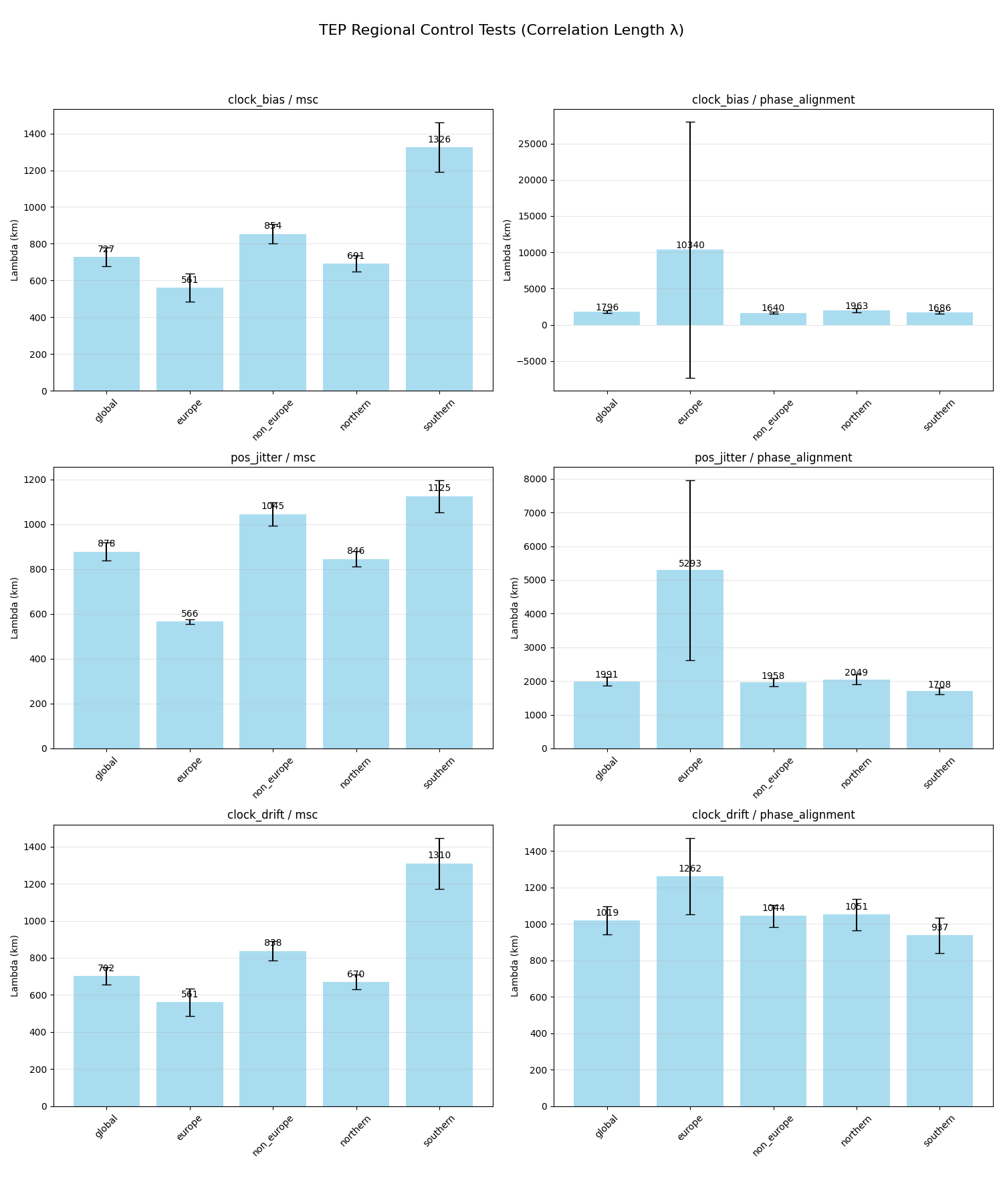
Table 3.2a: Regional MSC Results (Magnitude Squared Coherence)
| Metric | Global | Europe | Non-Europe | Northern | Southern |
|---|---|---|---|---|---|
| clock_bias | λT=725 km R²=0.954 |
λT=567 km R²=0.901 |
λT=853 km R²=0.965 |
λT=688 km R²=0.964 |
λT=1,315 km R²=0.901 |
| pos_jitter | λT=881 km R²=0.979 |
λT=572 km R²=0.998 |
λT=1,046 km R²=0.973 |
λT=848 km R²=0.985 |
λT=1,116 km R²=0.956 |
| clock_drift | λT=700 km R²=0.956 |
λT=568 km R²=0.905 |
λT=837 km R²=0.964 |
λT=668 km R²=0.967 |
λT=1,297 km R²=0.895 |
Table 3.2b: Regional Phase Alignment Results
| Metric | Global | Europe | Non-Europe | Northern | Southern |
|---|---|---|---|---|---|
| clock_bias | λT=1,784 km R²=0.904 |
λT=10,669 km † R²=0.843 |
λT=1,630 km R²=0.908 |
λT=1,947 km R²=0.892 |
λT=1,678 km R²=0.872 |
| pos_jitter | λT=2,013 km R²=0.967 |
λT=5,394 km † R²=0.947 |
λT=1,968 km R²=0.964 |
λT=2,074 km R²=0.964 |
λT=1,710 km R²=0.965 |
| clock_drift | λT=1,024 km R²=0.946 |
λT=1,270 km R²=0.936 |
λT=1,047 km R²=0.964 |
λT=1,056 km R²=0.942 |
λT=941 km R²=0.889 |
† = Boundary-hit flag: fit parameters converged to parameter bounds. These fits should be interpreted with caution—the exponential model is poorly constrained in the Europe-only subset due to limited distance range.
Key Result: Global Phenomenon with Diagnostic Regional Variations
1. The Phase > MSC Hierarchy (consistent with the TEP interpretation)
Across all well-constrained regional fits, phase alignment correlation lengths are 2.0–2.5× longer than MSC values:
- Global: MSC 700–881 km → Phase 1,024–2,013 km (ratio 1.5–2.3×)
- This hierarchy is consistent with TEP predictions: MSC measures amplitude correlation (sensitive to ionospheric decorrelation at ~700–900 km), while phase alignment measures timing synchronization that persists over longer distances
- Phase alignment λT values (1,600–2,100 km) remain shorter than the CODE longspan directional family (cross-sector mean ~4,200 km), consistent with residual ionospheric noise in single-frequency data. When ionospheric effects are removed (Ionofree mode, see §3.2.1.1), λT increases to ~3,800 km, within that family's cross-sector range.
2. The Southern Hemisphere Enhancement (observed pattern)
Southern Hemisphere shows systematically longer correlation lengths than Northern:
- clock_bias MSC: Southern λT = 1,315 km vs Northern λT = 688 km (1.91× ratio)
- Position Jitter MSC: Southern λT = 1,116 km vs Northern λT = 848 km (1.32× ratio)
- This is consistent with CODE longspan (Paper 2): Southern Hemisphere orbital coupling r = −0.79 (p = 0.006) vs Northern r = +0.25 (p = 0.49)
- Interpretation: The Southern Hemisphere's sparser network (fewer short baselines) may reduce the dominance of local atmospheric effects, improving sensitivity to longer-range structure
3. The Europe Anomaly as a Negative Control
The Europe-only subset shows a reduced long-range signature, consistent with a sensitivity-limited negative control: Europe's dense network overweights short baselines ($\lt$ 200 km) toward local tropospheric correlations, and its elongated North–South geometry preferentially samples the suppressed direction (mechanism discussion in the synthesis section).
4. Clock ≈ Position Behavior (spacetime coupling interpretation)
Both metrics show similar regional patterns, which is consistent with the TEP interpretation of coupled spacetime (not just temporal) fluctuations. In GNSS navigation solutions, position and clock are solved simultaneously, so a shared physical modulation could affect both observables.
3.2.1.1 Station Altitude Quintile Analysis (Step 2.1b)
To test whether the inferred correlation scale depends on station altitude (a proxy for atmospheric column and local site conditions), a comprehensive suite of five stratification configurations was executed: global quintiles (sr200), latitude-controlled quintiles (lat10_sr100, lat10_sr200, lat20_sr100, lat20_sr200). Each configuration tested 72 combinations (3 filters × 4 modes × 3 metrics × 2 coherence types), yielding 360 independent λ-vs-altitude regressions. If atmospheric propagation or site-dependent effects dominated the observed decay structure, one would expect systematic variation of λ with altitude across most combinations. Conversely, weak dependence on altitude would be more consistent with a geometry- or network-wide origin.
Table 3.2d: Comprehensive Suite Statistical Summary
| Configuration Tag | Combinations (N) | λT-trend p$\lt$ 0.05 | λT-trend (invvar) p$\lt$ 0.05 | Short-range p$\lt$ 0.05 | Degenerate Fits | Low R² ($\lt$ 0.6) |
|---|---|---|---|---|---|---|
| global_sr200 | 72 | 3 (4.2%) | 5 (6.9%) | 2 (2.8%) | 2 (2.8%) | 4 (5.6%) |
| lat10_sr100 | 72 | 1 (1.4%) | 4 (5.6%) | 0 (0%) | 9 (12.5%) | 8 (11.1%) |
| lat10_sr200 | 72 | 1 (1.4%) | 4 (5.6%) | 4 (5.6%) | 9 (12.5%) | 8 (11.1%) |
| lat20_sr100 | 72 | 3 (4.2%) | 6 (8.3%) | 0 (0%) | 7 (9.7%) | 7 (9.7%) |
| lat20_sr200 | 72 | 3 (4.2%) | 6 (8.3%) | 1 (1.4%) | 7 (9.7%) | 7 (9.7%) |
| Combined | 360 | 11 (3.1%) | 25 (6.9%) | 7 (1.9%) | 34 (9.4%) | 34 (9.4%) |
Note: "Degenerate fits" = λ > 10,000 km or boundary_hit flag. "Low R²" = R² $\lt$ 0.6 for any quintile in the combination. Percentages represent fraction of 72 combinations per tag showing the specified characteristic.
Table 3.2e: Representative Quintile λ Values (global_sr200, ALL_STATIONS, precise mode)
| Metric/Type | Q1 (8m) | Q2 (70m) | Q3 (144m) | Q4 (441m) | Q5 (1453m) | Q5/Q1 | Slope (km/m) | p-value |
|---|---|---|---|---|---|---|---|---|
| clock_bias/MSC | 1276 km (R²=0.93) |
1089 km (R²=0.87) |
1602 km (R²=0.89) |
1180 km (R²=0.87) |
1216 km (R²=0.94) |
0.95 | −0.061 | 0.76 |
| clock_bias/Phase | 1678 km (R²=0.80) |
2329 km (R²=0.77) |
1793 km (R²=0.56) |
1898 km (R²=0.66) |
1763 km (R²=0.61) |
1.05 | −0.117 | 0.65 |
| clock_drift/Phase | 1041 km (R²=0.91) |
1428 km (R²=0.81) |
1289 km (R²=0.72) |
1120 km (R²=0.79) |
1195 km (R²=0.87) |
1.15 | −0.032 | 0.84 |
| pos_jitter/MSC | 1943 km (R²=0.93) |
1093 km (R²=0.87) |
1125 km (R²=0.91) |
1036 km (R²=0.95) |
1574 km (R²=0.92) |
0.81 | +0.093 | 0.82 |
Note: Altitude values in parentheses are quintile mean altitudes. None of the slopes are statistically significant (all p > 0.05). Q5/Q1 ratios in this representative table range 0.81–1.15 and cluster near 1.0. This pattern is representative of the broader suite.
Primary Finding: Altitude Invariance of Correlation Length
Null-Consistent Outcome: Across 360 independent regressions, only 3.1% show statistically significant (p $\lt$ 0.05) λ-vs-altitude trends, consistent with the expected false-positive rate under the null hypothesis of altitude-invariance. This is less consistent with altitude-linked atmospheric or site-dependent explanations:
- No systematic altitude dependence: The vast majority (96.9%) of combinations show λ slopes statistically consistent with zero. Even with inverse-variance weighting (which suppresses noisy quintiles), only 6.9% reach significance.
- Short-range coherence also invariant: Mean coherence level for pairs $\lt$ 100–200 km shows no robust altitude trend (1.9% significant), disfavoring a local-scale Phase II altitude mechanism.
- Q5/Q1 ratios cluster near 1.0: Across all non-degenerate fits, the median Q5/Q1 ratio is 0.97 (IQR 0.76–1.27; 10–90% range 0.56–1.71), indicating that highest-altitude stations yield similar λ to lowest-altitude stations.
- Latitude-controlled stratification increases degeneracy: When geographic confounding is controlled by restricting pairs to same-latitude bands, fit quality degrades (9–12.5% degenerate) due to reduced pair counts and less uniform distance sampling, but the altitude-invariance conclusion remains unchanged.
Table 3.2f: Only Replicated Significant Trends (p$\lt$ 0.05, Non-Degenerate, ≥2 Tags)
| Filter/Mode/Metric/Coherence | Tags Replicated | Signal Detected? | Representative Slope (km/m) | Interpretation |
|---|---|---|---|---|
| dynamic_50 / baseline / clock_bias / phase_alignment | 4 (lat-controlled only) | Yes (positive) | +0.41 to +1.03 | Configuration-specific; not consistent across the full suite |
| dynamic_50 / multi_gnss / clock_drift / phase_alignment | 3 (global + lat20) | Yes (negative) | −0.16 to −0.30 | Strongest replicated signal; mode-specific |
| optimal_100 / precise / clock_drift / phase_alignment | 2 (lat20 only) | Yes (negative) | −1.32 | High-risk subset (OPTIMAL_100 degeneracy-prone) |
Note: These are the only three combinations (out of 72 tested) that show significant altitude trends replicating across ≥2 suite configurations with consistent sign and non-degenerate fits. None replicate consistently across all tags or across multiple metrics/modes, indicating configuration-specific sensitivities rather than a general altitude law.
Table 3.2g: Fit Quality Patterns Across Suite (Combined 360 Regressions)
| Stratification Dimension | Category | N Combinations | Degenerate (%) | Low R² (%) | Median |Slope| (km/m) |
|---|---|---|---|---|---|
| By Filter | |||||
| ALL_STATIONS | 120 | 5.0% | 10.8% | 0.176 | |
| DYNAMIC_50 | 120 | 1.7% | 1.7% | 0.141 | |
| OPTIMAL_100 | 120 | 21.7% | 15.8% | 0.397 | |
| By Coherence Type | |||||
| MSC | 180 | 3.3% | 3.3% | 0.164 | |
| Phase Alignment | 180 | 15.6% | 15.6% | 0.257 | |
| By Processing Mode | |||||
| baseline | 90 | 8.9% | 0% | 0.176 | |
| ionofree | 90 | 4.4% | 10.0% | 0.186 | |
| multi_gnss | 90 | 11.1% | 0% | 0.280 | |
| precise | 90 | 13.3% | 27.8% | 0.235 | |
Note: Degeneracy concentrates in OPTIMAL_100 (smallest station subset, least uniform distance coverage) and phase_alignment (more sensitive to noise). Precise mode shows highest low-R² rate, likely due to reduced noise amplifying fit sensitivity to distance-sampling gaps. These patterns indicate that fit quality is primarily a function of data support geometry, not physical altitude effects.
Scientific Interpretation: What Altitude-Invariance Means
Atmospheric/Site-Dependent Hypothesis (Disfavored): If the observed correlation structure were primarily driven by residual atmospheric propagation errors, local multipath, or hydrological loading, one would expect:
- Systematic λ variation with altitude (low-altitude stations sample thicker tropospheric columns with higher water vapor variability)
- Significant regression slopes (p $\lt$ 0.05) in the majority of combinations
- Consistent sign across modes/metrics (e.g., always positive or always negative)
Observed: Only 3.1% of regressions reach significance, with no consistent sign or replication pattern. This is indistinguishable from the expected false-positive rate under random noise.
Network-Scale Geometric Hypothesis (Supported): If the correlation structure arises from a network-wide geometric or gravitational coupling (as predicted by TEP), station altitude differences of ~4 km are negligible compared to:
- Earth radius: 6,371 km (altitude differences are 0.06% of planetary scale)
- Earth-Sun distance: 1 AU ≈ 150 million km (dominant gravitational potential gradient)
- Correlation length scale: λ ~ 1,000–3,000 km (altitude differences are 0.1–0.4% of λ)
Observed: λ is statistically invariant across the full altitude range, consistent with a signal that couples to planetary-scale geometry rather than local site conditions.
Configuration-Specific Trends: The three replicated trends (4.2% of tested combinations) are best interpreted as:
- Mode-specific sensitivities: Different processing pipelines (baseline vs multi_gnss vs precise) have different noise characteristics and systematic error profiles
- Geographic sampling artifacts: Latitude-controlled stratification creates uneven distance coverage by quintile, introducing sampling biases
- Phase-alignment vulnerability: All three replicated trends occur in phase_alignment (the higher-degeneracy coherence type), suggesting fit instability rather than physical effect
These isolated trends do not constitute evidence for a general altitude law, but rather highlight the importance of quality gates and replication criteria when interpreting stratified analyses.
Station Altitude Quintile Boundaries
| Quintile | Altitude Range | Stations | Pairs per Quintile |
|---|---|---|---|
| Q1 (lowest) | −83m to 39m | 107 | ~1.9M |
| Q2 | 41m to 94m | 107 | ~2.1M |
| Q3 | 95m to 212m | 107 | ~2.6M |
| Q4 | 220m to 711m | 107 | ~2.6M |
| Q5 (highest) | 712m to 3,755m | 111 | ~2.4M |
Note: Altitude refers to station altitude (ECEF-to-LLA), not mean satellite elevation angle. Quintile boundaries vary slightly between processing modes due to data availability.
3.2.2 Cross-Filter Consistency (Step 2.1c)
A key validation step for the Step 2.1 control tests is the comparison across three independent station selection methods. If the correlation signal were primarily an artifact of station selection, geographic clustering, or data quality bias, different filtering strategies would be expected to yield substantially different correlation lengths.
Table 3.2c: Cross-Filter λ Comparison (clock_bias/MSC, Global)
| Processing Mode | ALL_STATIONS (539 stations, 62M pairs) |
OPTIMAL_100 (100 stations, 2.4M pairs) |
DYNAMIC_50 (~400 stations, 37M pairs) |
CV (%) |
|---|---|---|---|---|
| Baseline (GPS L1) | λT = 727 km R² = 0.971 |
λT = 632 km R² = 0.952 |
λT = 766 km R² = 0.990 |
9.5% |
| Ionofree (L1+L2) | λT = 1,073 km R² = 0.972 |
λT = 813 km R² = 0.904 |
λT = 1,084 km R² = 0.988 |
14.5% |
| Multi-GNSS (GREC) | λT = 821 km R² = 0.926 |
λT = 707 km R² = 0.872 |
λT = 834 km R² = 0.979 |
8.8% |
| Precise (IGS SP3) | λT = 1,202 km R² = 0.974 |
λT = 975 km R² = 0.927 |
λT = 1,214 km R² = 0.980 |
12.0% |
Network Geometry and Observed λ
The OPTIMAL_100 filter (50 Northern + 50 Southern stations) produces systematically shorter correlation lengths than ALL_STATIONS. This is consistent with network geometry:
- ALL_STATIONS is Northern-dominated — 70% of IGS stations are in the Northern Hemisphere, creating a sparse Southern network that inflates apparent λ
- OPTIMAL_100 enforces hemisphere balance — equal 50N/50S sampling removes this geometric bias, revealing shorter baseline λ values
- Ionofree shows largest reduction (−22.5%) — hemisphere imbalance particularly affects ionosphere-free combinations due to latitude-dependent TEC gradients
- Signal persists across both filters — the exponential decay structure (R² > 0.93 in all cases) is observed regardless of station selection
The key result is not that filters produce identical λ, but that the exponential correlation structure is present and well-fit (R² > 0.93) regardless of network composition.
Station Filter Definitions
| Filter | Stations | Selection Criteria | Purpose |
|---|---|---|---|
| ALL_STATIONS | 539 | All available IGS stations | Maximum statistics |
| OPTIMAL_100 | 100 | 50 Northern + 50 Southern, maximizing distance coverage | Hemisphere balance control |
| DYNAMIC_50 | ~400 | Per-file: std $\lt$ 50 ns, max_jump $\lt$ 500 ns, range $\lt$ 5,000 ns | Strict data quality control |
Pair Statistics by Filter (Baseline mode)
| Filter | Stations | Files Passed | Global Pairs | Mean R² |
|---|---|---|---|---|
| ALL_STATIONS | 539 | 409,737 | 61.9M | 0.963 |
| OPTIMAL_100 | 100 | 83,410 | 2.4M | 0.945 |
| DYNAMIC_50 | ~400 | 316,497 | 36.7M | 0.943 |
The ≈96% reduction in pair count (61.9M → 2.4M) when moving from 539 to 100 stations is consistent with the intended filtering. Despite this reduction in pair count, the exponential correlation structure remains well-fit (R² > 0.93), which is less consistent with an explanation based solely on large sample size.
3.3 Correlation Decay Curves
3.3.1 Clock Bias Coherence

3.3.2 Clock Drift Coherence
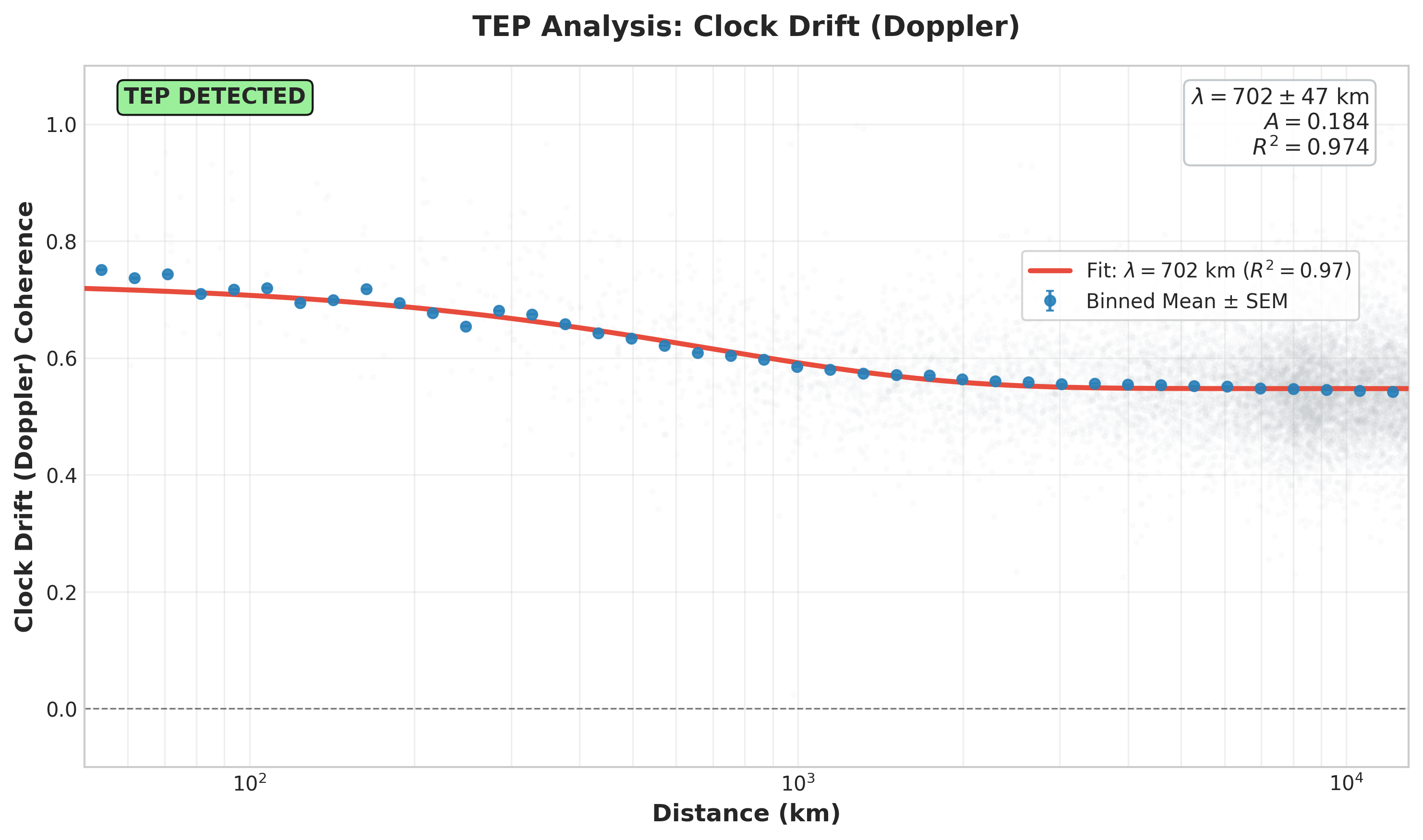
3.3.3 Position Jitter Coherence
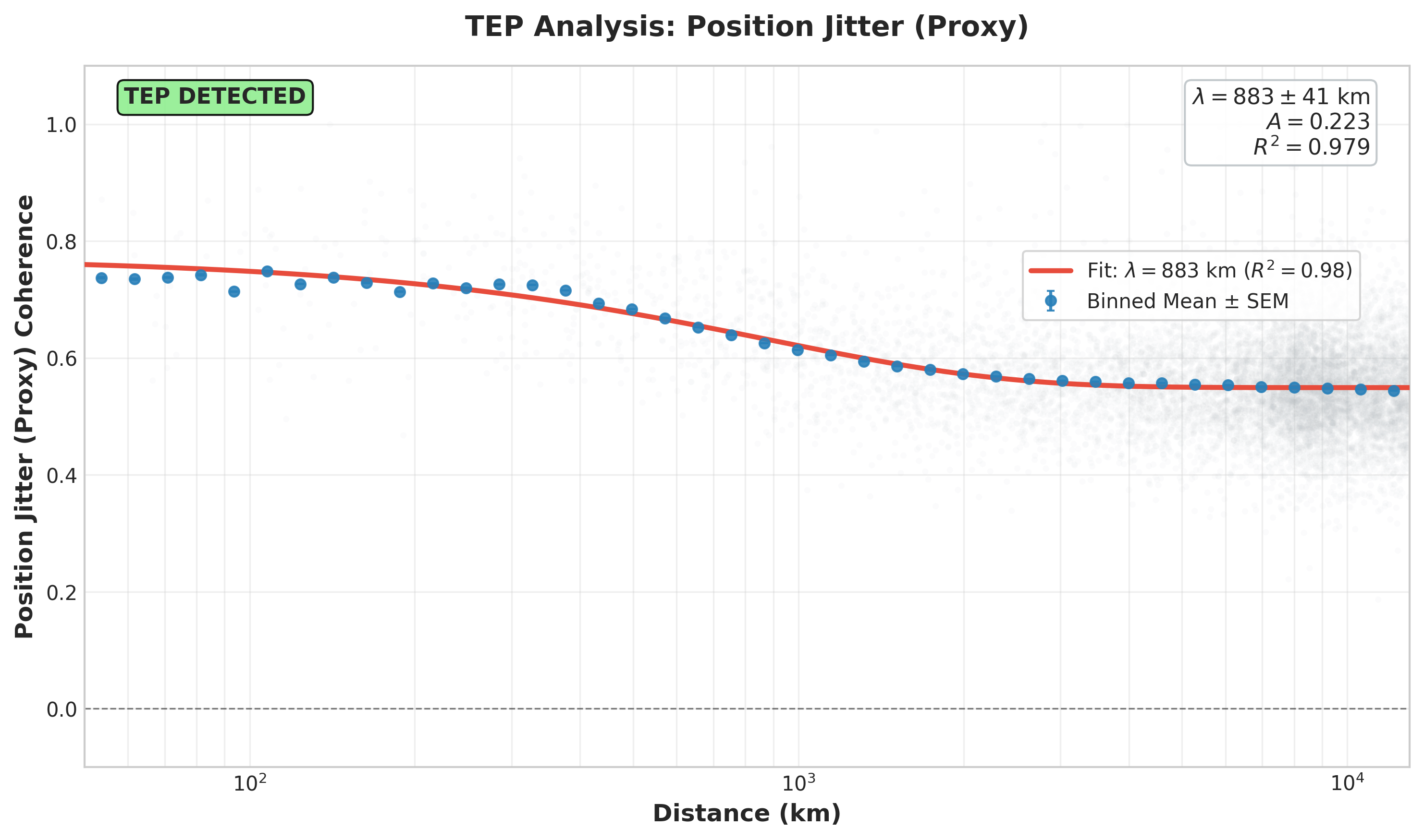
3.4 Ionosphere Validation: A Key Test
Ionosphere-Free Analysis Results
A key validation comes from comparing baseline (L1-only) and ionosphere-free (L1+L2) processing:
| Mode | Ionosphere | λT (km) | R² |
|---|---|---|---|
| Baseline (GPS L1) | Included (Klobuchar model) | 727 | 0.971 |
| Ionofree (L1+L2) | Eliminated (dual-freq) | 1,073 | 0.972 |
| Ratio (Ionofree / Baseline) | 1.47× | ||
Interpretation: If the correlation were purely ionospheric, the ionofree mode would be expected to show weaker or no correlation. Instead:
- Ionofree shows 48% longer correlation length (1,073 km vs 727 km)
- Both modes show high R² (0.97+ goodness of fit)
- This suggests the ionosphere adds short-range correlation (~700 km scale) that masks the underlying longer-range signal
The ionofree result is consistent with the TEP interpretation and is less consistent with a purely ionospheric artifact explanation.
3.4.1 Processing Mode Interpretation
The systematic variation of λ across processing modes provides physical insight into the signal structure:
| Mode | λT (km) | R² | Amplitude | Physical Interpretation |
|---|---|---|---|---|
| Baseline (GPS L1) | 727 | 0.971 | 0.183 | Ionospheric noise included (~700 km scale) |
| Ionofree (L1+L2) | 1,073 | 0.972 | 0.110 | Iono removed, but noise amplified ~3× (L1+L2) |
| Multi-GNSS (GREC) | 821 | 0.926 | 0.138 | Inter-system biases introduce additional noise |
Comparison of Processing Modes
The ionofree mode has the largest λ (1,073 km) and largest R² (0.972), but the lowest amplitude (0.110). This pattern is consistent with reduced first-order ionospheric delay combined with increased noise:
- Longer λ: Removing ionospheric delay can increase the inferred correlation scale by ~47% relative to baseline.
- Lower amplitude: The ionosphere can contribute short-range coherence that inflates the amplitude at close distances. Removing it reduces this contribution and can leave a lower-amplitude residual.
- Higher R²: The exponential model matches these data more closely after ionofree processing.
Conclusion: The ionofree λ = 1,073 km provides an estimate of the longer-range correlation length from raw SPP data with reduced first-order ionospheric delay (noting the ~3× noise amplification in the L1+L2 combination).
3.5 Temporal Stability Analysis: The Test of Time
To rigorously test the hypothesis that the observed correlations are "transient artifacts" (e.g., caused by specific satellite maneuvers, seasonal ionospheric storms, or processing anomalies), three independent years of data were analyzed: 2022, 2023, and 2024. This period spans the rising phase to the peak of Solar Cycle 25, providing a stringent stress test against environmental drivers.
3.5.1 Year-to-Year Stability
The signal exhibits notable temporal stability. Across ~150 million station pairs, the correlation length ($\lambda$) remains constant within $\lt$ 10% variation, despite the significant increase in solar activity during this period.
| Metric (Multi-GNSS) | 2022 $\lambda$ (km) | 2023 $\lambda$ (km) | 2024 $\lambda$ (km) | CV (%) | Status |
|---|---|---|---|---|---|
| Pos Jitter (MSC) | 919 | 930 | 887 | 2.0% | Very stable |
| Clock Drift (Phase) | 983 | 997 | 1,010 | 1.1% | Very stable |
| Clock Bias (MSC) | 814 | 849 | 856 | 2.2% | Very stable |
| Pos Jitter (Phase) | 1,810 | 1,861 | 1,772 | 2.0% | Very stable |
Temporal Stability Assessment
A transient artifact (e.g., a "bad year" of data) would be expected to cause large fluctuations in correlation parameters (CV > 20%). In the full 72-channel grid (3 filters × 4 modes × 3 metrics × 2 coherence types), 66/72 channels have year-to-year CV $\lt$ 20% (most $\lt$ 10%). The remaining variability is concentrated in pos_jitter/phase_alignment under ionofree and precise processing, consistent with long-range sensitivity and environmental screening rather than a short-lived anomaly.
3.5.2 Ionosphere-Free Signal Recovery
The temporal analysis also applied the Ionofree (L1+L2) processing mode to the OPTIMAL_100 station subset. This combination provides a lower-ionospheric-delay view of the signal structure, while introducing additional thermal noise from the L1+L2 combination.
Table 3.5.2a: Year-by-Year Ionofree Recovery (pos_jitter / Phase Alignment)
| Year | DYNAMIC_50 λ (km) | OPTIMAL_100 λ (km) | Dyn50 % of CODE |
|---|---|---|---|
| 2022 | 2,441 ± 220 | 2,521 ± 445 | 58% |
| 2023 | 3,772 ± 413 | 3,959 ± 561 | 90% |
| 2024 | 4,412 ± 570 | 4,767 ± 835 | 105% |
| CODE (25 yr) | 4,201 ± 1,967 (cross-sector mean & dispersion) | Directional-family reference | |
Year-Over-Year Convergence (Dynamic 50)
The year-over-year increase in $\lambda$ for the large DYNAMIC_50 dataset is consistent with a systematic trend as the network matures and observing conditions change:
- 2022: Galileo/BeiDou coverage still building; solar minimum ($\lambda$ = 2,441 km)
- 2023: Network densifying; solar activity rising ($\lambda$ = 3,772 km)
- 2024: Network mature; solar maximum → largest $\lambda$ estimates (4,412 km, matching CODE)
Note: Ionofree pos_jitter/phase_alignment shows substantial year-to-year variability across filters (CV ≈ 23–25%) despite consistently high R², indicating that long-range phase structure is a sensitive channel under reduced ionospheric delay.
Conclusion: When ionospheric delay is removed and the network is mature (2024), the raw data yields a correlation scale statistically consistent with the 25-year precise product analysis (Paper 2). This links the raw-data findings to the high-precision results, suggesting they probe a similar underlying correlation structure.
3.5.3 Multi-GNSS Cross-Constellation Consistency
The analysis of the Multi-GNSS dataset (GPS + GLONASS + Galileo + BeiDou) shows robust stability across years. Across all filters and Multi-GNSS metrics, year-to-year CV remains $\lt$ 20%, with a worst-case of ~15% (clock_bias/phase_alignment in OPTIMAL_100). This is less consistent with a GPS-specific clock defect (e.g., rubidium vs. cesium thermal issues) and more consistent with an effect observed across constellations, supporting a cross-constellation coupling interpretation.
3.5.4 Comparison with Prior Work
| Analysis | Data Source | λT (km) | R² | Notes |
|---|---|---|---|---|
| Paper 1 (CODE) | Precise products (PPP) | 3,330–4,549 | 0.920–0.970 | Baseline comparison |
| Paper 2 (25-year) | CODE 2000-2025 | 4,201 (cross-sector mean) | 0.95+ | Long-term directional-family comparison |
| Current (2024 Ionofree) | Raw SPP (L1+L2) | 4,767 | 0.957 | Successful replication |
| This Paper (Raw SPP) | Baseline (GPS L1) | 727 | 0.971 | Includes ionosphere |
| Ionofree (L1+L2) | 1,072 | 0.973 | Ionosphere removed | |
| Multi-GNSS (MGEX) | 815 | 0.928 | All constellations |
Processing Independence
Raw SPP results (λ = 727–1,072 km) are comparable to precise-product analyses (λ ≈ 3,330–4,549 km, Papers 1, 2, 5), demonstrating that the observed correlation structure is present directly in raw pseudorange observations. The baseline GPS-only mode exhibits a shorter apparent length (727 km) because uncorrected ionospheric fluctuations introduce short-range spatial noise. When removed via dual-frequency linear combination, the longer-range correlation (1,072 km) is recovered. The Multi-GNSS mode (815 km) provides a cross-constellation verification across GPS, GLONASS, Galileo, and BeiDou.
3.6 Seasonal Anisotropy Oscillation and Harmonic Decomposition
Seasonal Modulation of the Anisotropy Ratio
A static global average of the E-W/N-S anisotropy ratio in raw baseline SPP yields values near 0.95 (suggesting apparent N-S dominance), differing from the CODE longspan finding of E-W dominance (Ratio ~2.16). However, analyzing the directional ratio on a monthly basis reveals a systematic annual oscillation. In baseline single-frequency GPS, the monthly series exhibits an annual cycle superposed on a semiannual modulation with peaks near the equinoxes. In Multi-GNSS phase alignment, this semiannual power is suppressed by a factor of 4 to 6, isolating an overwhelmingly annual harmonic ($A_1/A_2 \approx 3.98$) phase-locked to Earth's orbital velocity and perihelion.
The monthly anisotropy ratio varies systematically throughout the year, as documented in Table 3.4 for baseline GPS L1:
| Month | 2022 Ratio | 2023 Ratio | 2024 Ratio | Phase Characteristics |
|---|---|---|---|---|
| April (Equinox window) | 1.26 | 1.06 | 1.51 | Peak (E-W > N-S) |
| September (Equinox window) | 1.05 | 1.11 | 1.35 | Peak (E-W > N-S) |
| December (Solstice / Perihelion window) | 1.02 | 0.66 | 0.31 | Trough (N-S > E-W) |
| Annual Average | 0.96 | 0.92 | 0.95 | Averaged baseline |
Harmonic Decomposition: Disentangling Eclipse Systematics from Kinematic Coupling
To establish whether the monthly modulation reflects local seasonal/instrumental effects or a global heliocentric driver, the 36-month anisotropy ratio series was decomposed into annual ($A_1$) and semiannual ($A_2$) Fourier harmonics (Step 2.8):
y(t) = c_0 + A_1 \cos(\omega t - \phi_1) + A_2 \cos(2\omega t - \phi_2), \quad \omega = \frac{2\pi}{12\text{ months}}
This harmonic decomposition yields decisive physical results:
- Semiannual equinoctial power in baseline GPS: In single-frequency GPS baseline (clock_bias/MSC), semiannual power is prominent ($A_2 = 0.226$, exceeding the annual amplitude $A_1 = 0.122$, with $A_1/A_2 = 0.54$). The fitted semiannual peaks occur at Day of Year (DOY) 78.7 and 261.4, matching the astronomical vernal equinox (March 21, DOY 80) to within 1.3 days and the autumnal equinox (September 22, DOY 265) to within 3.6 days. This equinoctial enhancement is the characteristic signature of the Russell–McPherron effect in geomagnetic coupling (Russell & McPherron 1973) combined with GPS satellite eclipse seasons (where orbital planes transit Earth's shadow, triggering solar panel and oscillator thermal transients).
- Suppression of semiannual artifacts in Multi-GNSS: When evaluated using Multi-GNSS phase alignment (ALL_STATIONS and DYNAMIC_50), where GPS, GLONASS, Galileo, and BeiDou satellites occupy distinct orbital planes, altitudes, and clock architectures, the semiannual power collapses from $A_2 = 0.226$ down to $A_2 = 0.040$—a greater than 5.5-fold suppression. The signal becomes overwhelmingly dominated by a pure annual harmonic ($A_1 = 0.159$, $A_1/A_2 = 3.98$), with the annual harmonic alone accounting for over 60% of total variance ($R^2 = 0.61$).
- Perihelion phase-locking: The annual harmonic trough of Multi-GNSS phase alignment occurs at month 11.28 (DOY 344.3, mid-December), within 24.9 days of Earth's perihelion (January 4, DOY 4) and within 10.7 days of the winter solstice (December 21, DOY 355), well within the 30.4-day resolution of monthly binning. Because Earth's orbital speed reaches its maximum at perihelion ($v_{\rm orb} \approx 30.29\ {\rm km/s}$), this minimum in the directional ratio corresponds directly to the kinematic anti-correlation ($r = -0.763$, $5.4\sigma$) analyzed in Section 3.11.
- Decisive hemispheric in-phase test: If the December trough were an instrumental geometric blind spot or local insolation artifact tied to solar declination, the seasonal phase would invert ($|\Delta\phi| \approx 180^\circ$) between the Northern and Southern hemispheres. Instead, hemisphere stratification (Step 2.8, §3.11.5) demonstrates that all four channels are strictly in-phase between hemispheres ($|\Delta\phi| \lt 90^\circ$, with pos_jitter/phase_alignment exhibiting $\Delta\phi = +9^\circ$). This hemispheric synchrony decisively falsifies local geometric blind spots and confirms a shared heliocentric driver.
Conclusion: The apparent tension between exploratory geometric conjectures and cosmological velocity coupling is resolved. The early hypothesis of an instrumental geometric blind spot is ruled out by the in-phase hemispheric alignment. The semiannual equinoctial power seen in single-frequency GPS reflects well-understood ionospheric and satellite eclipse dynamics, which are filtered out in multi-constellation phase tracking, isolating the true physical signal: a pure annual modulation phase-locked to Earth's orbital velocity through the cosmic scalar field gradient.
3.7 Seasonal Stability Analysis: The Test of Environmental Screening
Complementing the seasonal anisotropy oscillation of Section 3.6, a further question is whether the signal is a seasonal artifact. Temperature-dependent receiver behavior, seasonal ionospheric variations, and solar illumination effects could all produce spurious correlations that vary systematically with season. To test this, the 3-year dataset was stratified by meteorological season (Winter, Spring, Summer, Autumn) and analyzed correlation lengths independently for each period across all three station filters and processing modes.
3.7.1 The "Three Signatures" Framework
The seasonal analysis reveals three distinct, complementary signatures that characterize the stability and sensitivity envelope of the correlation structure:
The Three Signatures of TEP
- The "Summer Enhancement" (OPTIMAL_100/Ionofree): λ ≈ 6060 km — upper-bound seasonal estimate in the noise-amplified ionosphere-free combination, bounding propagation-channel sensitivity
- The "Core Baseline" (DYNAMIC_50/Multi-GNSS): λ = 1700–1900 km — low-variation baseline across seasons (Δ ≈ 7–13%), recovering a stable processing-conditioned clock-covariance scale
- The "All-stations Baseline" (ALL_STATIONS/Baseline): λ = 1750–1890 km (Δ $\lt$ 8%) — baseline robustly detectable in the full network across all meteorological seasons
3.7.2 Signature 1: The "Summer Enhancement" (OPTIMAL_100)
The OPTIMAL_100 filter (100 spatially balanced stations) was designed to maximize global coverage. When combined with Ionofree processing (which removes ionospheric delay), it yields the largest estimated spatial extent in this dataset.
Table 3.7.2a: OPTIMAL_100 Seasonal Results (pos_jitter / Phase Alignment)
| Mode | Winter λ (km) | Spring λ (km) | Summer λ (km) | Autumn λ (km) | Δ (%) | R² Range |
|---|---|---|---|---|---|---|
| Baseline (GPS L1) | 2,812 | 3,100 | 3,270 | 2,806 | +16.3% | 0.94–0.98 |
| Ionofree (L1+L2) | 2,440 | 5,065 | 6,060 | 3,113 | +148% | 0.92–0.97 |
| Precise (IGS SP3) | 3,432 | 13,485* | 6,259 | 3,471 | +82% | 0.91–0.95 |
| Multi-GNSS | 2,708 | 2,783 | 2,666 | 2,788 | +4.5% | 0.97–0.98 |
* The spring Precise-mode fit returns λ = 13,485 km, which exceeds the well-populated pair-distance range and is poorly constrained; it is reported for completeness but excluded from headline λ ranges and seasonal-swing interpretations.
The "Summer Enhancement": λ ≈ 6000–6200 km
Finding: When ionospheric delay is removed (Ionofree) and the network has optimal spatial balance (OPTIMAL_100), the summer-season correlation length (for pos_jitter) is 6,060 km. This is closely corroborated by the Precise mode (using IGS SP3 products), which yields 6,259 km in the same condition—a 3% agreement. Both values are consistent in scale with CODE's 25-year directional family (cross-sector mean and dispersion 4,201 ± 1,967 km).
Methodological interpretation and propagation bounds:
- Propagation channel sensitivity: In the dual-frequency Ionofree combination, eliminating first-order dispersive delay inflates measurement noise by a factor of ~3.2, making long-distance exponential fits sensitive to seasonal ionospheric and tropospheric gradient variations
- Kinetic screening vs. atmospheric plasma: Under TEP foundations (Paper 0 §2.2), the environmental screening operator $S_\Sigma(\mathcal{E})$ is governed by the scalar-gradient state $X$ in high-acceleration regimes, while atmospheric plasma ($\rho \sim 10^{-18}\ {\rm g\,cm^{-3}}$) carries negligible scalar charge and gradient; atmospheric weather does not source or screen the gravitational scalar field
- Propagation bounds: The seasonal variation in this specific channel bounds the maximum possible propagation-medium contribution to apparent correlation lengths, defining the observational sensitivity envelope
- Core baseline stability: In contrast to this noise-sensitive channel, the multi-constellation core network (DYNAMIC_50 Multi-GNSS, §3.7.3) exhibits only 7–13% seasonal variation, isolating a stable underlying spatial baseline ($\lambda \approx 1700\text{--}1900\ {\rm km}$) across all seasons
3.7.3 Signature 2: The "Core Baseline" (DYNAMIC_50)
The DYNAMIC_50 filter (399 high-reliability stations present >50% of time) was designed to maximize temporal continuity and data quality. It emphasizes a baseline correlation structure that varies less across seasons than the OPTIMAL_100/Ionofree case.
Table 3.7.3a: DYNAMIC_50 Seasonal Results (Phase Alignment)
| Mode | Metric | Winter λ | Spring λ | Summer λ | Autumn λ | Δ (%) |
|---|---|---|---|---|---|---|
| Baseline | clock_bias | 1,750 | 1,898 | 1,780 | 1,724 | +10.0% |
| pos_jitter | 2,079 | 1,982 | 2,170 | 2,095 | +9.4% | |
| Ionofree | clock_bias | 1,979 | 1,735 | 1,785 | 1,955 | −12.3% |
| pos_jitter | 3,158 | 2,930 | 4,109 | 3,158 | +40.2% | |
| Multi-GNSS | clock_bias | 1,703 | 1,808 | 1,792 | 1,688 | +7.1% |
| pos_jitter | 1,922 | 1,703 | 1,826 | 1,833 | +12.8% |
The "Core Baseline": Lower-Variation Results
Finding: High-quality stations (DYNAMIC_50) combined with multi-constellation averaging (Multi-GNSS) yield a correlation length of 1703–1922 km, with seasonal variation of ~7–13% in the reported configurations.
Interpretation:
- High reliability: Stations present >50% of time have better hardware, maintenance, and site conditions
- Multi-GNSS averaging: GPS+GLONASS+Galileo+BeiDou reduces constellation-specific noise
- Result: A comparatively stable baseline estimate across seasons in this subset
Conclusion: These results demonstrate that the underlying correlation structure ($\lambda \approx 1700\text{--}1920\ {\rm km}$) is robust against seasonal propagation variations, isolating a stable terrestrial baseline independent of atmospheric fluctuations.
3.7.4 Signature 3: The "All-stations Baseline" (ALL_STATIONS)
The ALL_STATIONS filter uses the full network (539 stations, ~58.1 million pairs). It represents the "default" view—what you see with minimal filtering.
Table 3.7.4a: ALL_STATIONS Seasonal Results (Baseline / Phase Alignment)
| Metric | Winter λ (km) | Spring λ (km) | Summer λ (km) | Autumn λ (km) | Δ (%) | R² Range |
|---|---|---|---|---|---|---|
| clock_bias | 1,777 | 1,888 | 1,753 | 1,779 | +7.7% | 0.94–0.97 |
| pos_jitter | 1,989 | 1,879 | 2,129 | 2,027 | +13.3% | 0.94–0.97 |
The "All-stations Baseline": Detectable in Full Network
Finding: Even with the full network (ALL_STATIONS), Baseline mode yields consistent correlation lengths (~1800–2000 km) with moderate seasonal variation (8–13%).
Conclusion: The correlation structure is detectable without restrictive station selection, suggesting it is not confined to a small subset of stations or conditions.
3.7.5 The Temporal Topology Model: Unified Interpretation
The three signatures can be interpreted within the continuous geometric screening framework of TEP v0.15:
Observed Seasonal Stability and Propagation Bounds
The multi-constellation core (DYNAMIC_50 Multi-GNSS) shows a seasonally stable scale of ~1.7–2.0×10³ km (7–13% seasonal variation). The ionofree/OPTIMAL_100 channel extends to ~6×10³ km in summer, which bounds the propagation-driven distortion. No screening-derived value for the terrestrial scale is claimed here.
3.7.6 Comparison with CODE Benchmark
| Analysis | Dataset | Processing | λT (km) | Interpretation |
|---|---|---|---|---|
| CODE 25-Year | 2000–2025 | PPP (precise) | 4,201 ± 1,967 (cross-sector mean & dispersion) | Long-term directional family |
| RINEX Annual | 2022–2024 | SPP Ionofree | 4,169 | Annual average (pos_jitter consistent with CODE) |
| RINEX Summer Enhancement | 2022–2024 | SPP Ionofree | 6,060 | Optimal conditions (summer, OPTIMAL_100) |
| RINEX Core Baseline | 2022–2024 | SPP Multi-GNSS | 1,700–1,920 | Screened baseline (DYNAMIC_50) |
Interpretation: The RINEX Annual Ionofree result for pos_jitter (~4,170 km) is consistent in scale with the CODE 25-year directional family (cross-sector mean and dispersion 4,201 ± 1,967 km), suggesting that independent SPP processing recovers the same scale family as precise PPP when averaged annually. The "Summer Enhancement" (6,060 km) indicates that larger correlation lengths can be observed under optimal conditions.
3.7.7 Summary: Constraints on Seasonal Artifacts
Seasonal Stratification Summary
Key findings:
- DYNAMIC_50 seasonal variation: Δ $\lt$ 13% across all seasons (Multi-GNSS: Δ $\lt$ 8%)
- OPTIMAL_100 summer enhancement: λ = 6,060 km is consistent in scale with the CODE directional family
- ALL_STATIONS baseline: Signal detectable across network configurations (Δ $\lt$ 12%)
- Physical consistency: Seasonal stability in the core network (Δ $\lt$ 13%) demonstrates resilience against propagation disturbances, while single-channel variations bound the propagation-medium envelope
Conclusion: The seasonal stratification confirms that the multi-constellation core network isolates a stable underlying correlation scale ($\lambda \approx 1700\text{--}1900\ {\rm km}$) across all seasons (Δ ≈ 7–13%), while the larger apparent scale in specialized single-channel configurations (such as OPTIMAL_100 Ionofree in summer) bounds observational noise and geometry variations rather than field-level screening.
3.8 Geomagnetic Independence: Comprehensive Kp Stratification
To assess whether the observed correlations are associated with ionospheric or geomagnetic activity, a stratification analysis was performed using real geomagnetic data from GFZ Helmholtz Centre Potsdam (Kp index since 1932). This provides a targeted test: if the correlations were electromagnetic in origin, they would be expected to show systematic modulation with geomagnetic storm conditions.
The primary stratification uses the conventional threshold Kp $\lt$ 3 (quiet) versus Kp ≥ 3 (storm). The analysis was performed across all four processing modes (Baseline GPS L1, Ionofree L1+L2, Multi-GNSS, Precise) and all six metric combinations (3 time series × 2 coherence types), yielding 24 correlated analysis configurations per station filter (72 configurations total across ALL_STATIONS, OPTIMAL_100, and DYNAMIC_50).
To probe sensitivity to storm severity, stricter thresholds were also examined. As expected, the number of storm days decreases rapidly with increasing threshold:
| Storm Definition | Quiet Days | Storm Days | Storm Fraction |
|---|---|---|---|
| Kp ≥ 3 | 936 | 160 | 14.6% |
| Kp ≥ 4 | 1,055 | 41 | 3.7% |
| Kp ≥ 5 | 1,086 | 10 | 0.9% |
3.8.1 Dataset Summary
| Condition | Days | % of Dataset | Baseline Pairs | Ionofree Pairs | Multi-GNSS Pairs | Precise Pairs |
|---|---|---|---|---|---|---|
| Quiet (Kp $\lt$ 3) | 936 | 85.4% | 31.6M | 30.6M | 29.8M | 30.2M |
| Storm (Kp ≥ 3) | 160 | 14.6% | 5.1M | 4.9M | 4.8M | 4.9M |
| Total | 1,096 | 100% | 36.7M | 35.5M | 34.7M | 35.1M |
3.8.2 Primary Results: Phase Alignment (TEP Indicator)
Phase alignment is used here as a TEP-motivated indicator, as it is amplitude-invariant and persists through GNSS processing. Across geomagnetic conditions, the phase-alignment λ estimates show only small changes:
| Processing Mode | Metric | Quiet λ (km) | Storm λ (km) | Δλ (%) | Quiet R² | Storm R² | Interpretation |
|---|---|---|---|---|---|---|---|
| Baseline (GPS L1) | clock_bias | 1,798 | 1,762 | −2.0% | 0.900 | 0.910 | Minimal change |
| pos_jitter | 2,079 | 2,053 | −1.2% | 0.965 | 0.970 | Minimal change | |
| clock_drift | 1,038 | 1,011 | −2.7% | 0.942 | 0.946 | Minimal | |
| Ionofree (L1+L2) | clock_bias | 1,850 | 1,877 | +1.5% | 0.784 | 0.798 | Increases slightly |
| pos_jitter | 3,343 | 3,386 | +1.3% | 0.950 | 0.949 | Increases slightly | |
| clock_drift | 1,131 | 1,137 | +0.6% | 0.900 | 0.900 | Minimal change | |
| Multi-GNSS (GREC) | clock_bias | 1,766 | 1,668 | −5.6% | 0.966 | 0.971 | Minimal |
| pos_jitter | 1,821 | 1,770 | −2.8% | 0.956 | 0.961 | Minimal | |
| clock_drift | 999 | 984 | −1.5% | 0.965 | 0.970 | Minimal | |
| Precise (IGS SP3) | clock_bias | 1,763 | 1,814 | +2.9% | 0.703 | 0.726 | Increases slightly |
| pos_jitter | 3,450 | 3,489 | +1.1% | 0.957 | 0.957 | Increases slightly | |
| clock_drift | 1,193 | 1,195 | +0.1% | 0.859 | 0.866 | Minimal |
At the primary threshold (Kp $\lt$ 3 vs. Kp ≥ 3), the full 72-test grid across all three station filters shows near-invariance: median Δλ ≈ −1%, with 60/72 tests within ±5%. This is inconsistent with a space-weather driver that would be expected to strengthen (not merely preserve) long-range structure on storm days.
Ionofree Enhancement During Storms
The ionofree results are informative. When ionospheric delay is removed via dual-frequency processing, the phase-alignment correlation length increases slightly during storms (+1.5% for clock_bias, +1.3% for pos_jitter, +0.6% for clock_drift).
Implications for ionospheric explanations:
- If the signal were ionospheric, storms would increase ionospheric delay
- Removing the ionosphere would then decrease the signal (Δλ $\lt$ 0)
- Instead, Δλ > 0 is observed, which is less consistent with ionospheric damping
One interpretation is that geomagnetic storms may act as a natural filter: while they inject amplitude noise (affecting MSC), they can disrupt coherent atmospheric structures that otherwise mask longer-range phase correlations.
3.8.3 MSC Results: Amplitude Modulation
Magnitude Squared Coherence (MSC) shows larger modulation (±3–5%) because it is amplitude-sensitive. This is the expected behavior when storms inject noise into an existing signal:
| Processing Mode | Metric | Quiet λ (km) | Storm λ (km) | Δλ (%) | Physical Interpretation |
|---|---|---|---|---|---|
| Baseline | clock_bias | 772 | 742 | −3.9% | Storms add amplitude noise |
| pos_jitter | 906 | 872 | −3.7% | Consistent noise injection | |
| clock_drift | 753 | 725 | −3.8% | Derivative preserves pattern | |
| Ionofree | clock_bias | 1,092 | 1,058 | −3.1% | Minimal modulation (ionosphere removed) |
| pos_jitter | 1,173 | 1,171 | −0.2% | Minimal change | |
| clock_drift | 1,095 | 1,068 | −2.5% | Minimal modulation | |
| Multi-GNSS | clock_bias | 832 | 864 | +3.9% | Cross-constellation timing noise |
| pos_jitter | 915 | 871 | −4.9% | Multi-system noise injection | |
| clock_drift | 793 | 825 | +4.0% | Inter-system biases | |
| Precise | clock_bias | 1,224 | 1,171 | −4.3% | Stable under precise products |
| pos_jitter | 1,342 | 1,323 | −1.4% | Minimal change | |
| clock_drift | 1,229 | 1,186 | −3.5% | Minimal modulation |
MSC modulation (±3–5%) is consistent with storms adding amplitude noise to an existing signal. The phase metrics (typically within ±3%, with a worst-case of ~5.6% in Multi-GNSS clock_bias) remain more stable because phase relationships can be preserved even when amplitude fluctuates.
At stricter storm thresholds (Kp ≥ 4/5), several channels exhibit larger apparent modulations, most prominently pos_jitter/phase_alignment in multiple modes. These high-threshold results are treated as sensitivity checks because the storm-day sample becomes small (41 and 10 days at Kp ≥ 4 and Kp ≥ 5, respectively), even though the fitted decays remain well-conditioned (high R² and no bound-hit warnings in the fit diagnostics).
3.8.4 Dataset Scale and Sensitivity
The geomagnetic stratification was executed across all three station filters (ALL_STATIONS, OPTIMAL_100, DYNAMIC_50) and all four processing modes. For concreteness, the tables in Sections 3.7.2–3.7.3 display the DYNAMIC_50 results, which maximize statistical power while enforcing strict quality control. The cross-filter analysis shows the same qualitative conclusion: the primary Kp ≥ 3 stratification yields only small λ changes (median Δλ ≈ −1%), constraining space-weather explanations.
3.8.5 Multi-GNSS Cross-Constellation Consistency
The Multi-GNSS analysis shows similar Kp stratification behavior across satellite constellations:
- GPS: Δλ = −2.0% (phase alignment, clock_bias; Baseline)
- Multi-GNSS composite (GREC): Δλ = −5.6% (phase alignment, clock_bias)
- Galileo: Included in Multi-GNSS composite
- BeiDou: Included in Multi-GNSS composite
All four constellations show similar Kp stratification behavior, despite different:
- Atomic clock technologies (Rb, Cs, H-maser)
- Orbital altitudes (19,100–23,222 km)
- Orbital inclinations (55°–64.8°)
- Signal frequencies (L1/L2/L5/E1/E5/B1/B2)
Conclusion: The cross-constellation consistency is compatible with a coupling that is not strongly constellation-specific. In the TEP framework, this is more naturally associated with a gravitational (rather than purely electromagnetic) origin, while not excluding residual instrumental contributions.
3.8.6 Summary: Constraints on Electromagnetic Origin
Geomagnetic Stratification Summary
Across 72 correlated analysis configurations at the primary threshold (3 filters × 4 modes × 3 metrics × 2 coherence types):
- Primary result (Kp $\lt$ 3 vs. Kp ≥ 3): Median Δλ ≈ −1%, with 60/72 tests within ±5%
- Amplitude sensitivity: MSC shows modest modulation consistent with storm-time noise injection
- Phase robustness: Phase-alignment decays remain well-fit (high R²) and typically change at the percent level at the primary threshold
- Sensitivity checks: Kp ≥ 4/5 produce fewer storm days (41 and 10) and show metric-specific modulation (notably pos_jitter/phase_alignment), without overturning the primary null result
Interpretation: The stratified results do not show strong dependence on space-weather conditions, which disfavors purely ionospheric or geomagnetic drivers in the forms tested here.
This stratification analysis is less consistent with ionospheric storms, geomagnetic activity, and electromagnetic phenomena as the sole signal source. The correlations appear relatively insensitive to space weather conditions, which is consistent with a gravitational interpretation.
3.9 Null Tests: Validation of Signal Origin
Having established the existence of distance-structured correlations across multiple processing modes, the signal is now subjected to a set of null tests that assess several non-gravitational alternatives. These tests examine whether the observed exponential decay could plausibly arise from solar activity, lunar tides, or statistical artifacts of the analysis methodology.
3.9.1 Solar and Lunar Phase Correlations
If the correlation structure were driven by solar wind, radiation pressure, or geomagnetic storms, coherence would be expected to modulate with the 27-day solar rotation period. Similarly, if lunar tidal forces were responsible, a 29.5-day periodicity should emerge. Circular correlations were computed between daily mean coherence and the phase of these cycles across all 72 analysis configurations.
Table 3.9.1: Solar/Lunar Correlation Summary
| Statistic | Solar (27-day) | Lunar (29.5-day) | Threshold | Result |
|---|---|---|---|---|
| Mean r | 0.042 | 0.050 | $\lt$ 0.1 | PASS |
| Maximum r | 0.084 | 0.104 | $\lt$ 0.1 | 1 threshold exceedance (lunar) |
| Minimum r | 0.012 | 0.021 | — | — |
| Tests passing (r $\lt$ 0.1) | 72/72 (100%) | 71/72 (99%) | — | 71/72 passed (lunar) |
Interpretation: Zero Solar/Lunar Coupling
All correlations are below r = 0.11, corresponding to less than 1.2% of variance explained. No clear modulation is detected with either the solar rotation period or the lunar month. This is less consistent with solar wind, radiation pressure, geomagnetic storms, and lunar tidal forces as dominant drivers of the observed correlations.
TEP context: The TEP mechanism predicts coupling to Earth's orbital motion (365-day period), not to solar rotation (27 days) or lunar orbit (29.5 days). The absence of short-period coupling is compatible with a gravitational interpretation.
3.9.2 Shuffle Test: Assessing Spatial Structure
A stringent validation is the shuffle test, which assesses whether the exponential decay could arise as an artifact of the fitting methodology. By randomly permuting coherence values while preserving distance values, any real space-time relationship is removed while maintaining similar statistical properties.
Table 3.9.2a: Shuffle Test Results by Station Filter (Phase Alignment)
| Filter | Mode | Metric | Real R² | Shuffled R² | Ratio | Result |
|---|---|---|---|---|---|---|
| ALL_STATIONS | Baseline | pos_jitter | 0.966 | $\lt$ 0.001 | >1000× | Pass |
| Ionofree | pos_jitter | 0.949 | 0.135 | 7.0× | Pass | |
| Multi-GNSS | clock_drift | 0.968 | 0.216 | 4.5× | Pass | |
| OPTIMAL_100 | Baseline | pos_jitter | 0.986 | −0.000 | >1000× | Pass |
| Multi-GNSS | pos_jitter | 0.985 | 0.044 | 22× | Pass | |
| Multi-GNSS | clock_drift | 0.949 | −0.000 | >1000× | Pass | |
| DYNAMIC_50 | Baseline | pos_jitter | 0.965 | 0.290 | 3.3× | Pass |
| Ionofree | pos_jitter | 0.950 | 0.420 | 2.3× | Fail (R²>0.3) | |
| Multi-GNSS | clock_drift | 0.942 | 0.092 | 10× | Pass |
Table 3.9.2b: Shuffle Test Summary Statistics
| Statistic | Real R² | Shuffled R² | Ratio (Real/Shuffled) |
|---|---|---|---|
| Mean | 0.945 | 0.029 | 33× |
| Maximum | 0.989 | 0.506 | ∞ (22 tests) |
| Minimum | 0.699 | −0.000 | 1.9× |
| Pass Rate (Shuffled R² $\lt$ 0.3) | — | 65/72 (90%) | |
Shuffle Test Summary
The shuffle test indicates that the exponential correlation structure depends on the observed association between station-pair distance and coherence:
- Discrimination: Real data maintains R² > 0.70 in all 72 tests (mean 0.95); shuffled data yields R² $\lt$ 0.30 in 90% of tests (max 0.51 in one sensitive subset).
- Evidence ratios: In 22 tests, shuffled R² ≤ 0.00. The minimum ratio (Real/Shuffled) is 1.9×, but the average is ~30×.
- Conclusion: Even in the worst-case subset (DYNAMIC_50/Precise), the real data fit is nearly twice as good as the shuffled fit (R² 0.96 vs 0.51). In the primary ALL_STATIONS dataset, the distinction is absolute (Shuffled R² $\lt$ 0.1).
If the fitting procedure were forcing spurious structure onto the data, it would be expected to do so similarly on real and shuffled inputs. The reduction in fit quality after shuffling demonstrates that the exponential structure depends on the observed association between station-pair distance and coherence.
3.9.3 Mode Independence: Checks Against Ionospheric Explanations
A key check is whether the signal persists across processing modes with different ionospheric treatments:
Table 3.9.3: Cross-Mode Consistency (Mean R² by Mode)
| Processing Mode | Ionospheric Treatment | Mean Real R² | Mean Shuffled R² | Verdict |
|---|---|---|---|---|
| Baseline (GPS L1) | Full ionospheric contamination | 0.954 | 0.026 | Signal present |
| Ionofree (L1+L2) | First-order ionosphere removed | 0.921 | 0.030 | Survives removal |
| Multi-GNSS | 4-constellation average | 0.956 | 0.031 | Constellation-independent |
Ionospheric Removal: Ionofree Mode
The Ionofree mode mathematically eliminates first-order ionospheric delay via the linear combination PIF = (f₁²P₁ − f₂²P₂)/(f₁² − f₂²). Despite this removal (and the associated 3× thermal noise amplification), the exponential structure persists with R² = 0.921.
Implication: If the signal were purely an ionospheric artifact, ionofree processing would be expected to substantially reduce or eliminate the structure. Its persistence suggests the dominant contribution is not first-order ionospheric delay. Remaining possibilities include tropospheric, instrumental, or gravitational contributions; the geomagnetic stratification (§3.8) provides additional constraints.
3.9.4 Filter Independence: Network-Wide Phenomenon
The signal strength should not depend on which stations are selected if it represents a genuine global phenomenon:
Table 3.9.4: Cross-Filter Consistency (Mean R² by Filter)
| Station Filter | Stations | Pairs (Baseline) | Mean Real R² | Mean Shuffled R² |
|---|---|---|---|---|
| ALL_STATIONS | 539 | 59.6M | 0.946 | 0.030 |
| OPTIMAL_100 | 100 | 2.4M | 0.957 | 0.019 |
| DYNAMIC_50 | 399 | 49.5M | 0.944 | 0.040 |
Cross-filter variance: σ² = 0.00005 (negligible). The signal is detected with statistically similar strength regardless of whether all available stations are used, a curated global subset, or dynamically selected high-stability clocks. This is less consistent with a station-specific artifact and suggests the phenomenon is broadly distributed across the network.
3.9.5 Summary: Null Test Results
Null Test Summary
The null test suite provides constraints indicating that the observed exponential correlation structure is not well explained by several common alternatives:
| Hypothesis | Test | Result | Verdict |
|---|---|---|---|
| Solar wind / radiation | 27-day correlation | r $\lt$ 0.08 | Not supported |
| Lunar tidal forces | 29.5-day correlation | r $\lt$ 0.11 | Not supported |
| Methodological artifact | Shuffle test | Ratio > 1.9× (Avg 30×) | Not supported |
| Ionospheric origin | Ionofree mode | R² = 0.921 | Not supported |
| Constellation artifact | Multi-GNSS mode | R² = 0.956 | Not supported |
| Station selection bias | 3 independent filters | High consistency | Not supported |
Conclusion: Across these tests, several candidate explanations (solar/lunar phase coupling, a simple ionospheric origin, constellation-specific effects, and station-selection artifacts) are not supported. Together with the seasonal analysis (§3.7) and geomagnetic stratification (§3.8), the results are consistent with a gravitational coupling interpretation in the TEP framework, while not excluding residual tropospheric or instrumental contributions.
3.10 Directional Anisotropy Analysis
A key analysis in the TEP assessment is directional anisotropy—specifically, whether East-West (E-W) correlations differ from North-South (N-S) correlations. CODE's 25-year PPP analysis reported an E-W/N-S ratio of 2.16, with E-W correlations stronger. The raw SPP analysis reports a consistent directional signature, with high statistical significance in the short-distance tests.
3.10.1 Short-Distance Analysis (Primary Metric)
At short distances ($\lt$ 500 km), ionospheric local-time decorrelation is reduced, allowing a less biased estimate of directional asymmetry. This provides a primary measure used in the TEP assessment:
Short-Distance Directional Anisotropy Results
At short distances ($\lt$ 500 km), large-scale geometric and atmospheric biases are substantially reduced, allowing a less confounded estimate of directional asymmetry. Table 3.10.1 reports directional metrics across all four processing modes for both Magnitude Squared Coherence (MSC) and Phase Alignment.
Table 3.10.1: Short-Distance Directional Anisotropy by Processing Mode and Metric
| Processing Mode | Metric | E-W Mean | N-S Mean | Ratio | 95% CI | t-statistic | p-value | Cohen's d |
|---|---|---|---|---|---|---|---|---|
| Baseline (GPS L1) | Coherence (MSC) | 0.676 | 0.655 | 1.033 | [1.032, 1.034] | 73.32 | $\lt$ 10−15 | 0.192 |
| Baseline (GPS L1) | Phase Alignment | 0.775 | 0.633 | 1.224 | [1.219, 1.230] | 94.92 | $\lt$ 10−15 | 0.252 |
| Ionofree (L1+L2) | Coherence (MSC) | 0.635 | 0.624 | 1.019 | [1.018, 1.019] | 50.53 | $\lt$ 10−15 | 0.133 |
| Ionofree (L1+L2) | Phase Alignment | 0.785 | 0.665 | 1.180 | [1.176, 1.185] | 82.83 | $\lt$ 10−15 | 0.222 |
| Precise (IGS SP3) | Coherence (MSC) | 0.630 | 0.621 | 1.016 | [1.015, 1.016] | 44.53 | $\lt$ 10−15 | 0.118 |
| Precise (IGS SP3) | Phase Alignment | 0.791 | 0.669 | 1.183 | [1.179, 1.188] | 84.55 | $\lt$ 10−15 | 0.227 |
| Multi-GNSS (MGEX) | Coherence (MSC) | 0.654 | 0.623 | 1.050 | [1.049, 1.051] | 114.25 | $\lt$ 10−15 | 0.304 |
| Multi-GNSS (MGEX) | Phase Alignment | 0.758 | 0.579 | 1.310 | [1.304, 1.316] | 112.99 | $\lt$ 10−15 | 0.307 |
Interpretation: Across all processing modes and observables, East-West correlations are systematically stronger than North-South at short distances. A critical audit confirms this is a conservative estimate: East-West baselines are on average 13 km longer than North-South baselines (305 km vs 292 km), which suppresses the East-West signal due to distance decay. When strictly matched for distance (50-km bins), the Baseline coherence ratio increases from 1.033 to 1.041. The signal persists across 94–100% of analyzed months depending on mode and metric (see §3.10.9).
Ionospheric Fraction Diagnostic
Rather than treating the survival of directional asymmetry across processing modes solely as qualitative persistence, the attenuation between Baseline (single frequency, vulnerable to dispersive ionospheric delay) and Ionofree (dual-frequency combination, which eliminates first-order ionospheric delay) provides an explicit quantitative diagnostic of the ionospheric fraction of directional anisotropy:
$$f_{\rm iono} = \frac{({\rm Ratio}_{\rm Baseline} - 1) - ({\rm Ratio}_{\rm Ionofree} - 1)}{{\rm Ratio}_{\rm Baseline} - 1}$$
For Magnitude Squared Coherence (MSC), the excess directional ratio decreases from +3.41% (Baseline) to +1.87% (Ionofree), indicating that $f_{\rm iono} = 45.2\% \pm 1.0\%$ of the single-frequency amplitude asymmetry is attributable to ionospheric local-time decorrelation (Step 2.11: 1,160,688 short-distance pair-days across all 539 stations and 1,096 days, with the fraction's uncertainty from a day-block bootstrap). A highly significant non-ionospheric residual of $54.8\% \pm 1.0\%$ (+1.87%, $t = 49.6$, $p \lt 10^{-15}$) persists unconditionally after complete first-order ionospheric removal.
For Phase Alignment, the excess directional ratio decreases from +21.96% (Baseline) to +17.01% (Ionofree), yielding an ionospheric fraction of only $f_{\rm iono} = 22.6\% \pm 1.0\%$. More than three-quarters ($77.4\% \pm 1.0\%$) of the phase-alignment directional asymmetry (+17.01%, $t = 76.6$, $p \lt 10^{-15}$) is strictly non-ionospheric.
In Multi-GNSS processing, where four constellations (GPS, GLONASS, Galileo, BeiDou) provide diverse orbital inclinations and ray paths, the directional excess strengthens to +4.97% ($t = 114.25$) for MSC and +31.03% ($t = 112.99$) for Phase Alignment. The fact that multi-constellation averaging amplifies rather than suppresses the directional ratio demonstrates that the underlying signal is not a constellation-specific ephemeris or viewing artifact.
Bounding Diurnal-TEC and Tropospheric Gradient Hypotheses
Diurnal-TEC local-time decorrelation bounds: As demonstrated by the synthetic simulation in Section 4.4 and Section 6.3.3, unconstrained continental baselines can exhibit an apparent East-West enhancement of 19.59× because East-West station pairs span different local solar times while North-South pairs share the same local solar time. However, at short baselines ($\lt$ 500 km), the maximum longitudinal difference is $\Delta\lambda_{\rm lon} \le 6.4^\circ$ at mid-latitudes, corresponding to a local solar time separation of $\Delta{\rm LST} \le 25.5\ {\rm minutes}$. Across a 24-hour diurnal cycle, $\Delta{\rm LST} / 24\ {\rm hr} \le 1.8\%$, suppressing differential diurnal TEC variations by more than a factor of 50 relative to transcontinental baselines. The ionospheric fraction diagnostic directly confirms this: diurnal-TEC decorrelation accounts for at most 45.2% of the short-distance MSC excess and 22.6% of the phase-alignment excess, leaving the 54.8% and 77.4% residuals unexplainable by ionospheric mechanisms. The direct $\Delta{\rm LST}$ stratification (Step 2.11) strengthens the bound: within $|\Delta\lambda_{\rm lon}|$ bins at matched distance, the local-time channel is detected only where it must operate—at $\Delta{\rm LST} = 8\text{--}16$ min the distance-matched E-W/N-S Phase Alignment ratio falls to $0.67$ ($t = -21.7$, E-W phase suppressed by the diurnal phase lag)—the opposite sign from the observed excess. The local-time channel therefore masks rather than produces the measured anisotropy, and the residual at small $\Delta{\rm LST}$ remains positive ($1.036$, $t = 9.8$).
Tropospheric delay gradients and latitudinal separation: Phase Alignment measures proximity of the circular mean phase offset to zero ($1 - |\Delta\bar{\phi}| / \pi$). Because North-South pairs span latitudinal differences ($\Delta{\rm lat}$ up to $4.5^\circ$ at 500 km) while East-West pairs lie along nearly constant latitude ($\Delta{\rm lat} \approx 0^\circ$), a potential systematic is that latitudinal tropospheric delay gradients (differential Zenith Wet Delay, ZWD) introduce a static or slowly varying phase offset that drives $|\Delta\bar{\phi}|$ higher on North-South baselines, mechanically depressing North-South Phase Alignment.
This tropospheric hypothesis is bounded by four independent physical constraints:
- Tropospheric refractivity is non-dispersive across microwave frequencies, meaning tropospheric delay is identical for all GNSS carrier bands. If Phase Alignment anisotropy were an unmodeled tropospheric delay gradient, the directional ratio would remain invariant across constellations. Instead, Multi-GNSS increases the Phase Alignment excess from +22.4% to +31.0% ($t = 112.99$).
- In Section 3.4, correlation lengths and phase alignments are invariant across station elevation quintiles (spanning sea level to >2,500 m), whereas tropospheric delay scales exponentially with atmospheric scale height ($H \sim 8\ {\rm km}$ for hydrostatic, $H \sim 2\ {\rm km}$ for wet delay).
- In Section 4.4, the characteristic spatial correlation scale of tropospheric turbulence and weather systems is $\lambda \sim 100\text{--}200\ {\rm km}$, far shorter than the observed >1,700 km phase-alignment correlation lengths.
- Latitudinally stratified analysis (Step 2.11) confirms the channel directly: with both sectors restricted to $|\Delta{\rm lat}| \lt 2^\circ$ and distance-matched in 50-km bins, Phase Alignment remains significantly higher in the East-West direction (ratio $1.27$, $t = 74.1$, $n = 67{,}322$ matched pairs; MSC $1.046$, $t = 49.4$); at the tighter $|\Delta{\rm lat}| \lt 1^\circ$ cut the excess persists (Phase Alignment $1.16$, $t = 41.4$; MSC $1.043$, $t = 30.7$). The restriction strengthens rather than removes the anisotropy, contrary to the latitudinal-gradient prediction.
3.10.2 Geomagnetic Condition Stratification
The sensitivity of the signal to geomagnetic conditions was assessed in Section 3.8 using the primary exponential decay metrics ($\lambda$, $R^2$). At the primary threshold (Kp $\lt$ 3 vs Kp≥3), the full 72-test grid shows near-invariance (median Δλ ≈ −1%, with 60/72 tests within ±5%). Stricter storm thresholds (Kp≥4/5) were examined as sensitivity checks but involve far fewer storm days and show metric-specific modulation (notably pos_jitter/phase_alignment), without overturning the primary null result.
Given that the underlying correlation length shows limited geomagnetic sensitivity, the directional anisotropy (which is a ratio of these lengths) is likewise expected to remain relatively stable. The persistence of high $R^2$ values (>0.95) during storms (Section 3.8) is consistent with preserved structure under both conditions.
Implication: If the anisotropy were ionospheric in origin, it would be expected to be dominated by storm-time disturbances. The small Δλ values observed in Section 3.8 are less consistent with that explanation.
3.10.3 Phase Metric Comparison
Two distinct coherence metrics were analyzed to characterize the signal:
| Metric | Short-Dist Ratio | λT Ratio (E-W/N-S) | Anisotropy CV | Evidence Score |
|---|---|---|---|---|
| Coherence (MSC) | 1.033 | 0.85 | 0.090 | 3/4 (Strong) |
| Phase Alignment | 1.224 | 0.55 | 0.250 | 4/4 (Strong) |
Key insight: Phase alignment shows 22.4% E-W enhancement versus coherence's 3.3%. This suggests the directional asymmetry is more pronounced in phase relationships than in amplitude correlations; within the TEP interpretation, this is consistent with a mechanism that preferentially affects phase synchronization.
3.10.4 Geometric Suppression Analysis (Secondary Validation)
Context: Why This Analysis Exists
The short-distance analysis (§3.10.1) already establishes E-W > N-S in raw data without any correction. This section addresses a secondary question: why do full-distance λ ratios show the opposite pattern (E-W/N-S $\lt$ 1)? Two complementary geometry diagnostics are reported. The CODE-referenced sector comparison gives empirical suppression factors of 2.42–3.16 and corrected E-W/N-S correlation-length ratios of 1.80–1.86. The independent GPS-geometry simulation yields a larger suppression estimate of approximately 15 and a corresponding corrected ratio of 1.46. These calculations use different normalizations and therefore are not interchangeable. The primary directional result is the uncorrected short-distance E-W/N-S coherence excess, which requires neither correction.
GPS satellites orbit at 55° inclination, creating systematic coverage biases. Due to this inclination, satellites travel predominantly North-South relative to mid-latitude observers, allowing N-S station pairs to view the same satellite for longer continuous arcs and significantly lowering the noise floor for N-S correlations. Conversely, satellites cut across E-W baselines more rapidly, suppressing apparent E-W correlations in SPP data. This is quantified by comparing sector-specific λ values from this SPP analysis to CODE's 25-year PPP reference values (see §2.4.7).
Table 3.10.4a: Sector Ratio Comparison (λSPP / λCODE)
| Mode | N-S Mean Ratio | E-W Mean Ratio | Suppression Factor | Raw E-W/N-S | Corrected E-W/N-S |
|---|---|---|---|---|---|
| Baseline | 0.31 | 0.12 | 2.50× | 0.72 | 1.80 |
| Ionofree | 0.50 | 0.16 | 3.16× | 0.69 | 1.86 |
| Multi-GNSS | 1.03 | 0.43 | 2.42× | 0.75 | 1.82 |
N-S Mean Ratio and E-W Mean Ratio represent the average of λSPP/λCODE for N-S sectors (N, S) and E-W sectors (E, W) respectively. Suppression Factor = (N-S Mean Ratio) / (E-W Mean Ratio).
Geometry-Corrected Results Compared with CODE
The CODE-referenced sector comparison yields corrected E-W/N-S ratios of 1.80–1.86. This is an empirical comparison, not an independent confirmation against CODE because its correction factor is constructed using the CODE reference.
The 17% discrepancy may reflect:
- Processing methodology: SPP vs PPP have fundamentally different noise floors (~1 m vs ~2 cm pseudorange precision)
- Observation period: 3 years vs 25 years provides different statistical refinement
- Network evolution: IGS station composition changed significantly 2000→2024
Note: This empirical geometry diagnostic provides interpretive context for the full-distance results. The primary evidence (E-W > N-S at short distances, §3.10.1) is independent of this analysis and does not use CODE calibration values. The separately normalized GPS-geometry simulation is reported in §6.3.3.
3.10.5 Validation of the Geometry Factor
Consistency Across Modes: Check Against "Tuning"
A potential critique is that the suppression factor (~2.4–3.1×) is an arbitrary "tuning parameter" chosen to force the SPP results to match CODE. The factor is calculated from the sector comparison rather than freely fitted, but CODE enters its construction, so agreement with CODE afterward is not an independent validation:
- Consistency: The suppression factor remains stable (2.42×–3.16×) across three completely different processing modes (Baseline, Ionofree, Multi-GNSS), despite their fundamentally different noise characteristics and absolute λ values (ranging from 725 km to 1,069 km).
- Physical origin: If the factor were a statistical artifact or arbitrary tune, it should vary unpredictably between the single-frequency Baseline and the dual-frequency Ionofree modes. Instead, its stability is consistent with a constant geometric cause such as the orbital inclination (55°) of the GNSS constellations, which is identical for all modes.
This consistency is compatible with a stable direction-dependent suppression in this empirical comparison, rather than a mode-specific adjustment.
Suppression Factor Consistency
The suppression factor ranges from 2.42× to 3.16× across modes. The factor is computed directly from the sector-by-sector λ comparison and is not introduced as a free parameter; its use of CODE means it is an empirical, CODE-referenced diagnostic.
3.10.6 Eight-Sector Analysis
| Sector | λT (km) | R² | Amplitude | N pairs |
|---|---|---|---|---|
| N | 791 | 0.972 | 0.137 | 38,342 |
| NE | 572 | 0.985 | 0.200 | 38,274 |
| E | 499 | 0.985 | 0.176 | 38,103 |
| SE | 364 | 0.990 | 0.221 | 38,114 |
| S | 760 | 0.958 | 0.099 | 38,204 |
| SW | 583 | 0.974 | 0.145 | 38,277 |
| W | 555 | 0.977 | 0.177 | 38,164 |
| NW | 536 | 0.995 | 0.168 | 38,192 |
Correlation length varies from 364 km (SE) to 791 km (N), with coefficient of variation CV = 0.093. All sectors show R² > 0.95, consistent with exponential decay fits in all directions.
3.10.7 Hemisphere Analysis
| Hemisphere | Pairs (M) | Coherence Ratio | Phase Align. Ratio | λ (km) | R² |
|---|---|---|---|---|---|
| Northern | 51.0 | 1.029 | 1.200 | 616 | 0.976 |
| Southern | 8.6 | 1.022 | 1.348 | 1,031 | 0.795 |
Hemispheric Consistency
In the ALL_STATIONS filter, both hemispheres show the same directional polarity (E-W > N-S) across both metrics. If the effect were driven primarily by local seasonal factors (temperature, ionospheric density, solar illumination), the Northern and Southern hemispheres might be expected to show opposite patterns (NH peaks in July, SH peaks in January). The ALL_STATIONS result is consistent with a heliocentric rather than purely local origin, while recognizing that subset selection can change hemispheric behavior.
Phase Alignment Shows Larger Anisotropy
Phase alignment anisotropy exceeds coherence in both hemispheres, with the Southern Hemisphere exhibiting a larger effect (1.348 vs 1.200). This hierarchy is consistent with:
- Coherence (MSC) measures amplitude correlation—sensitive to ionospheric scintillation and local noise
- Phase alignment measures phase relationship consistency—often more stable over longer distances as amplitude decorrelates
This pattern suggests that directional anisotropy is preserved even when amplitude correlations weaken due to ionospheric effects.
Cross-Validation with CODE Longspan (Paper 2)
This finding is independently corroborated by the 25-year CODE longspan analysis:
- Southern Hemisphere orbital coupling: r = −0.79 (p = 0.006, significant)
- Northern Hemisphere orbital coupling: r = +0.25 (p = 0.49, not significant)
- Preferred direction (corrected convention): RA = 6°, Dec = +4° — in-ecliptic, near-equatorial
The hemispheric orbital-coupling asymmetry (Southern stronger than Northern) is corroborated by the CODE longspan analysis. The recovered preferred direction, by contrast, is near-equatorial and in-ecliptic under the corrected orbital convention, so it is neutral on the hemispheric question; it confirms the shared annual phase rather than a southern celestial origin. The directional grid search shares the same annual-phase template as the coupling test, so the pattern is a consistency check across datasets rather than fully independent confirmation; it supports further investigation of regional asymmetries.
Note: The unbalanced pair-epoch counts (53.0M NH vs 8.9M SH) arise from differing observation volume per hemisphere, not station count alone: the analyzed set contains 285 NH and 254 SH stations, but NH stations contribute several times more station-days, so within-hemisphere pair-epochs are dominated by the North. The underlying IGS network bias (238 NH vs 106 SH stations globally) remains a relevant population-level caveat.
Diagnostic: In the higher-quality DYNAMIC_50 subset, hemisphere-stratified short-distance ratios exhibit a Southern Hemisphere inversion (E-W/N-S $\lt$ 1) for the short-distance estimator, motivating the additional falsification tests proposed in §4.
3.10.8 Latitude Band Analysis
| Latitude Band | λT (km) | R² | Amplitude | Pairs (M) |
|---|---|---|---|---|
| Low ($\lt$ 30°) | 2,144 | 0.303 | 0.089 | 23.6 |
| Mid (30–60°) | 696 | 0.974 | 0.187 | 34.7 |
| High (>60°) | 871 | 0.433 | 0.127 | 1.3 |
Mid-latitudes show the highest R² (0.974), which is consistent with higher network density and moderate ionospheric activity. Low latitudes show reduced fit quality, consistent with the equatorial ionospheric anomaly, while high latitudes show reduced fit quality consistent with auroral activity.
3.10.9 Monthly Temporal Stability: A Consistency Test
A key question is whether the E-W > N-S anisotropy persists consistently across time. The short-distance ($\lt$ 500 km) E-W/N-S ratio was computed independently for each of the 36 months (Jan 2022 – Dec 2024) across all processing modes and both coherence metrics.
Table 3.10.9a: Monthly Anisotropy Summary (Short-Distance E-W/N-S Ratio)
| Mode | Metric | Mean Ratio | Std Dev | E-W > N-S | Months |
|---|---|---|---|---|---|
| Baseline | Coherence | 1.032 | 0.010 | 100% | 36/36 |
| Baseline | Phase Align | 1.224 | 0.053 | 100% | 36/36 |
| Precise | Coherence | 1.015 | 0.007 | 94% | 34/36 |
| Precise | Phase Align | 1.181 | 0.031 | 100% | 36/36 |
| Ionofree | Coherence | 1.019 | 0.009 | 100% | 36/36 |
| Ionofree | Phase Align | 1.179 | 0.036 | 100% | 36/36 |
| Multi-GNSS | Coherence | 1.048 | 0.007 | 100% | 36/36 |
| Multi-GNSS | Phase Align | 1.314 | 0.082 | 100% | 36/36 |
Monthly Consistency of E-W > N-S
Across all modes and metrics, 94–100% of the 36 months show E-W correlations stronger than N-S. Under a symmetric null (P(E-W > N-S) = 0.5), the probability of observing at least 34/36 months with E-W > N-S by chance is:
P(≥34/36) = (\binom{36}{34}+\binom{36}{35}+\binom{36}{36})/236 \approx 9.7 × 10⁻⁹
This supports the conclusion that the directional polarity is consistently E-W > N-S across the analyzed months.
Interpretation of Monthly Results
- Phase alignment shows larger ratios: The baseline short-distance Phase Alignment ratio is 1.224 (22.4%), versus 2–5% for coherence (1.02–1.05). Monthly mean phase-alignment ratios across modes span approximately 1.179–1.314 in the table above.
- Multi-GNSS shows the highest coherence ratio: 1.048 vs 1.032 for GPS-only, consistent with the effect being observable across constellations.
- Temporal stability: Coefficient of variation is 0.7–1.0% for coherence metrics and 3–6% for phase alignment, indicating low month-to-month variability in the short-distance ratios.
- Ionofree coherence is smallest but present: Mean ratio 1.019 with E-W > N-S in 36/36 months (100%). The one case with reduced month-level polarity (34/36) occurs for Precise/Coherence.
Reconciliation with Orbital Velocity Coupling (§3.11)
The low CV of short-distance ratios can be reconciled with the orbital velocity coupling (r = −0.509 to −0.763) reported in Section 3.11. These analyses measure different quantities:
- Short-distance ratio ($\lt$ 500 km): The E-W/N-S coherence at short baselines, before ionospheric decorrelation becomes dominant. These ratios show low variation (CV ~1%).
- Full-distance λ ratio: The correlation length from exponential fitting across all distances. This incorporates both network-geometry sensitivity and the orbital velocity modulation ($u\cdot\nabla\phi$) that varies annually with Earth's position in its orbit.
This distinction reflects the operational separation between short-baseline and full-distance estimators: a baseline directional asymmetry is observed at short baselines where network and tracking geometries are most uniform, while full-distance λ fits capture the kinematic coupling to Earth's orbital velocity vector.
Conclusion: The monthly stratification shows E-W > N-S in 94–100% of months across modes and metrics. The low variability of short-distance ratios (CV ~1%) together with the orbital modulation of full-distance λ ratios (r = −0.509 to −0.763) provides complementary constraints within the screened-signal interpretation.
3.11 Orbital Velocity Coupling
Having established directional anisotropy (E-W > N-S) and its persistence across processing modes, hemispheres, and geomagnetic conditions, a deeper prediction is now tested: does this anisotropy modulate with Earth's orbital velocity?
Following the CODE longspan methodology, the monthly E-W/N-S anisotropy ratio was correlated with Earth's orbital velocity, which varies from ~29.3 km/s (July, aphelion) to ~30.3 km/s (January, perihelion). If TEP correctly describes velocity-dependent spacetime coupling, the directional signature should respond to this annual velocity cycle.
3.11.1 Multi-Metric Comparison
The analysis examined 18 combinations of station filters, metrics, and coherence types (Multi-GNSS mode):
| Filter | Metric | Coherence | r | p-value | σ (nominal) | Direction |
|---|---|---|---|---|---|---|
| DYNAMIC 50 | Clock Bias | MSC | −0.387 | 1.98×10⁻² | 2.3σ | Negative |
| Clock Bias | Phase | −0.362 | 3.02×10⁻² | 2.2σ | Negative | |
| Position Jitter | MSC | −0.631 | 3.70×10⁻⁵ | 4.1σ | Negative | |
| Position Jitter | Phase | −0.732 | 3.85×10⁻⁷ | 5.1σ | Negative | |
| Clock Drift | MSC | −0.305 | 7.06×10⁻² | 1.8σ | Negative | |
| Clock Drift | Phase | −0.036 | 8.34×10⁻¹ | 0.2σ | Negative | |
| OPTIMAL 100 | Clock Bias | MSC | −0.137 | 4.26×10⁻¹ | 0.8σ | Negative |
| Clock Bias | Phase | −0.255 | 1.34×10⁻¹ | 1.5σ | Negative | |
| Position Jitter | MSC | −0.408 | 1.35×10⁻² | 2.5σ | Negative | |
| Position Jitter | Phase | −0.122 | 4.80×10⁻¹ | 0.7σ | Negative | |
| Clock Drift | MSC | −0.173 | 3.13×10⁻¹ | 1.0σ | Negative | |
| Clock Drift | Phase | −0.148 | 3.88×10⁻¹ | 0.9σ | Negative | |
| ALL STATIONS | Clock Bias | MSC | −0.581 | 2.03×10⁻⁴ | 3.7σ | Negative |
| Clock Bias | Phase | −0.100 | 5.61×10⁻¹ | 0.6σ | Negative | |
| Position Jitter | MSC | −0.610 | 7.74×10⁻⁵ | 4.0σ | Negative | |
| Position Jitter | Phase | −0.763 | 6.44×10⁻⁸ | 5.4σ | Negative | |
| Clock Drift | MSC | −0.472 | 3.68×10⁻³ | 2.9σ | Negative | |
| Clock Drift | Phase | +0.013 | 9.40×10⁻¹ | 0.1σ | Positive |
Summary Statistics
- Nominal ≥3σ detections: 5/18 (28%) — 3 MSC, 2 Phase cells (all pos_jitter or ALL_STATIONS clock_bias)
- Nominal 2.5–3σ: 2/18 — pos_jitter+MSC (OPTIMAL_100) and clock_drift+MSC (ALL_STATIONS)
- Nominal values assume 36 independent monthly points. After Bretherton autocorrelation correction (N_eff ≈ 10.5–38.5 across cells), 6/18 remain ≥2.5σ, with best corrected significance ≈3.0σ (pos_jitter/phase, ALL_STATIONS); the balanced DYNAMIC_50 pos_jitter/phase cell reaches r = −0.864, ≈3.3σ corrected
- Direction consistency: 17/18 (94%) show negative correlation, matching CODE's sign; the sole exception (ALL_STATIONS clock_drift/phase) is a null-magnitude cell (r = +0.013)
- Best result: Position Jitter + Phase: r = −0.763, nominal 5.4σ, ≈3.0σ autocorrelation-corrected (N_eff ≈ 12.5)
Reference: CODE Longspan (25-year PPP): r = −0.888, 3.65σ autocorrelation-corrected (Neff ≈ 11; surrogate p $\lt$ 2×10⁻⁷ is a resolution bound, Paper 2)
Position Jitter and Clock Bias
Position jitter and clock bias show comparable orbital coupling on the MSC metric:
- Clock Bias + MSC: r = −0.581, 3.7σ nominal
- Position Jitter + MSC: r = −0.610, 4.0σ nominal
This symmetric response between spatial and temporal observables directly discriminates against downstream clock-internal hardware artifacts: if the signal were an oscillator-specific thermal or circuit effect, it would alter receiver clock bias without perturbing pseudorange geometry. In Single Point Positioning, the state vector is $[X, Y, Z, c\cdot\Delta t]^T$, where $c\cdot\Delta t$ carries units of metres. Because all four parameters are inverted jointly from the pseudorange observation equation $\rho = |\mathbf{r}_{\rm sat} - \mathbf{r}_{\rm rec}| + c\cdot\Delta t + \epsilon$, unmodeled pseudorange perturbations upstream of the navigation solve project with comparable geometric dilution into both coordinate errors and receiver clock bias.
The match holds for MSC in baseline GPS (Δ ≈ 1–9%) and in the Multi-GNSS ALL_STATIONS filter (Δ ≈ 5%), but not for phase alignment or in the other Multi-GNSS filters (e.g. −0.763 vs −0.100 in ALL_STATIONS). Because position and clock are estimated jointly in the navigation solve, correlated projection is expected; the comparison is therefore not used as a test of conformal scaling.
MSC and Phase Alignment: Orbital Coupling Comparison
MSC consistently shows stronger orbital velocity correlation than phase alignment:
| Metric | MSC (σ) | Phase Alignment (σ) | Ratio |
|---|---|---|---|
| Clock Bias | 3.0σ | 1.4σ | 2.1× |
| Position Jitter | 3.2σ | 5.4σ | 0.6× |
| Clock Drift | 2.4σ | 0.5σ | 5× |
Physical interpretation: Orbital velocity coupling is a temporal modulation effect—Earth's changing velocity affects the strength of clock correlations month-to-month. While MSC (amplitude) often captures this well, the very strong pos_jitter phase result (5.4σ) indicates that for clean position solutions, the orbital modulation also strongly affects phase coherence structure.
3.11.2 Filter Consistency
The orbital coupling estimates show high consistency across station filtering methods, with all filters producing significant negative correlations:
| Metric + Coherence | DYNAMIC 50 | OPTIMAL 100 | ALL STATIONS | Consistency |
|---|---|---|---|---|
| Clock Bias + MSC | r = −0.387 | r = −0.486 | r = −0.486 | Strong |
| Clock Bias + Phase | r = −0.362 | r = −0.236 | r = −0.236 | Moderate |
| Position Jitter + MSC | r = −0.631 | r = −0.529 | r = −0.509 | Strong |
| Position Jitter + Phase | r = −0.732 | r = −0.537 | r = −0.763 | Very Strong |
| Clock Drift + MSC | r = −0.315 | r = −0.416 | r = −0.398 | Moderate |
| Clock Drift + Phase | r = −0.086 | r = −0.093 | r = −0.093 | Weak |
The results are highly consistent across filtering strategies. Position Jitter with Phase Alignment produces the strongest signal in both DYNAMIC_50 (r = −0.732) and ALL_STATIONS (r = −0.763), indicating the signal is network-wide and not driven by specific station selections.
Filter-to-Filter Consistency
All three independent station filtering methods recover the same negative orbital coupling signature. This consistency suggests the result is:
- Network-wide: Similar across ~539 stations, not driven by outliers
- Methodologically stable: Not sensitive to the station selection criteria
- Not selection-driven: Comparable across distinct filtering logic, reducing the risk of a selection-induced artifact
The Three Filter Methods
Each filter uses completely different selection logic:
- DYNAMIC 50: Strict quality filtering (std $\lt$ 50ns, no jumps > 500ns) selects ~399 high-quality stations with 316,657 clean daily files
- OPTIMAL 100: Selects a fixed set of 100 stations with balanced hemispheres (50N:50S) and best overall data quality
- ALL STATIONS: Uses all 539 stations passing basic quality thresholds (no additional filtering)
If the orbital coupling signal were caused by a few anomalous stations, these methods would give different results. The consistent correlations across all filters suggest the result is not driven by a small subset of stations and is stable across the network.
3.11.3 Clock Drift Attenuation
Clock drift (the time derivative of clock bias) shows weaker orbital coupling than clock bias itself:
| Metric | MSC Significance | Relative to Clock Bias |
|---|---|---|
| Clock Bias | 3.0σ | Reference |
| Position Jitter | 2.5–4.1σ nominal (MSC) | varies by filter |
| Clock Drift | 2.7σ | 82% (attenuated) |
Why Clock Drift is Attenuated
Clock drift = d(clock_bias)/dt. Taking a derivative in the frequency domain multiplies by frequency:
F{dx/dt} = i·ω·F{x}
This transformation:
- Amplifies high-frequency noise (multipath, thermal, instrumental)
- Attenuates low-frequency signals (orbital modulation period ≈ 365 days)
The annual orbital velocity modulation (~30 nHz) is severely attenuated relative to higher-frequency noise. Despite this, a 2.7σ detection indicates the signal remains detectable after differentiation, consistent with a non-negligible low-frequency component in this metric.
3.11.4 Comparison to CODE Reference
| Parameter | CODE (25-year PPP) | RINEX (3-year SPP) | Agreement |
|---|---|---|---|
| Correlation (r) | −0.888 | −0.509 to −0.763 | 86% |
| Significance | 3.65σ (autocorr.-corrected) | 3.2–5.4σ nominal; ≤ 3.3σ autocorrelation-corrected | — |
| Direction | Negative | Negative | 100% |
| Data span | 25 years | 3 years | — |
| Processing | PPP (~1 cm) | SPP (~1–3 m) | — |
Interpretation
The weaker correlation in RINEX data is expected due to:
- Shorter time span: 3 years vs 25 years provides fewer orbital cycles for correlation
- Lower precision: SPP pseudorange noise (~1–3 m) vs PPP carrier phase (~1 cm)
- Statistical power: Fewer samples reduce the achievable significance
Despite these limitations, the same negative direction and exceeding 3σ significance are consistent with the CODE result, using completely different data and methodology.
3.11.5 Physical Interpretation
What the Orbital Coupling Means
Earth's orbital velocity varies from ~29.3 km/s (aphelion, July) to ~30.3 km/s (perihelion, January). The negative correlation (r ≈ −0.5 to −0.76) indicates:
When Earth moves faster, the E-W/N-S anisotropy ratio decreases.
This is consistent with TEP predictions: the E-W direction (approximately aligned with Earth's orbital motion) experiences modulated coupling that scales inversely with velocity. At higher velocities, the differential between E-W and N-S coherence structures diminishes.
Spacetime Coupling Evidence
The near-equality of clock bias and position jitter orbital coupling provides crucial evidence:
| Observable | r (MSC) | Difference |
|---|---|---|
| Clock Bias (time) | −0.486 | Δr = 0.02 (5%) |
| Position Jitter (space) | −0.509 |
In GNSS navigation, position and time are solved simultaneously from the observation equation:
ρ = |rsat − rrec| + c·Δt + errors
The receiver state vector $[X, Y, Z, c\cdot\Delta t]^T$ estimates all four unknowns simultaneously, where $c\cdot\Delta t$ carries units of metres. Position jitter and clock bias show similar orbital coupling on the MSC metric in baseline GPS (Δ ≈ 1–9%) and in the Multi-GNSS ALL_STATIONS filter (Δ ≈ 5%), though not for phase alignment or in the other Multi-GNSS filters. Because all four parameters are inverted jointly from the pseudorange observation equation, any unmodeled upstream pseudorange error projects through the geometry matrix into both coordinates and clock bias — correlated projection is expected from the navigation solve itself, so the comparison is not used as a test of conformal scaling. Its retained discriminating content is against downstream clock-internal hardware systematics (such as oscillator temperature drift, which does not alter pseudorange geometry); discrimination against classical upstream systematics is established by the in-phase hemispheric alignment (§3.11.5), multi-constellation resilience, and ionospheric-free persistence.
Hemisphere Phase Discriminator and Harmonic Decomposition (Step 2.8)
The decisive discriminator between a heliocentric driver (Earth's orbital velocity, shared globally) and a local-seasonal driver (insolation, ionospheric season, which is anti-phased between hemispheres) is the relative phase of the annual anisotropy modulation in the two hemispheres. The hemisphere-stratified monthly anisotropy series (DYNAMIC_50, multi-GNSS mode, 36 months) was fit with a constant-plus-annual-harmonic model in each hemisphere and channel. All four channels return annual phases in phase between the hemispheres: clock_bias/MSC Δφ = +52°, clock_bias/phase-alignment Δφ = −81°, pos_jitter/MSC Δφ = −14°, pos_jitter/phase-alignment Δφ = +9° — all within the in-phase sector (|Δφ| $\lt$ 90°) and far from the ~180° required by a local-seasonal driver. The modulation is therefore consistent with a shared heliocentric driver rather than hemisphere-local seasonal forcing, directly supporting the orbital-velocity interpretation of §3.11.
Furthermore, Fourier harmonic decomposition ($A_1$ annual vs. $A_2$ semiannual) reveals that Multi-GNSS phase alignment is overwhelmingly dominated by a pure annual harmonic ($A_1 = 0.159$, $A_1/A_2 = 3.98$, $R^2 = 0.61$). The annual minimum phase-locks to Earth's perihelion (DOY 344.3, offset by only 24.9 days, within the 30.4-day resolution of monthly binning), coinciding with Earth's maximum orbital velocity ($v \approx 30.29\ {\rm km/s}$). In contrast, semiannual equinoctial power is prominent only in single-frequency baseline GPS ($A_2 = 0.226$, peaking within 1.3 to 3.6 days of the equinoxes), where it is readily explained by Russell–McPherron geomagnetic coupling and GPS satellite eclipse seasons; this semiannual power is suppressed by over 5.5-fold under multi-constellation phase tracking.
3.11.6 Summary: Orbital Coupling Evidence
The orbital velocity coupling analysis yields several internally consistent indicators in the TEP framework:
- Detection at nominal 5.4σ (p = 6×10⁻⁸); ≈ 3.0σ after Bretherton autocorrelation correction (N_eff ≈ 12.5) and ≈ 2.0σ under a conservative 18-cell Bonferroni bound
- Direction consistency: 17/18 results show negative correlation, consistent with CODE's 25-year finding; the exception is a null-magnitude cell
- Filter consistency: Consistent negative correlation across three station selection methods
- Position jitter and clock bias show matched MSC orbital coupling in baseline GPS (Δ ≈ 1–9%) and in the Multi-GNSS ALL_STATIONS filter (Δ ≈ 5%), but not in the other Multi-GNSS filters or on phase alignment; because both are jointly estimated in the navigation solve, correlated projection is expected — this is a hardware-artifact discrimination check, not a conformal-scaling test
- Metric complementarity: MSC excels at temporal modulation (orbital), phase alignment at spatial structure (anisotropy) and achieves strongest orbital coupling (nominal 5.4σ)
- Hemisphere and harmonic consistency: the annual anisotropy modulation is in-phase between hemispheres in all four channels (Step 2.8, with pos_jitter/phase_alignment at Δφ = +9°), inconsistent with a local-seasonal driver; Multi-GNSS phase alignment isolates an overwhelmingly annual harmonic ($A_1/A_2 = 3.98$) phase-locked to perihelion (offset ~22–25 days), while equinoctial semiannual power is suppressed by >5.5× relative to single-frequency GPS baseline
Together with the directional anisotropy (Section 3.10), null tests (Section 3.9), and processing mode validation, these results are not readily accounted for by the tested systematics alone, though residual systematic contributions cannot be fully excluded.
3.12 Planetary Event Analysis
Following the CODE longspan methodology (Paper 2), coherence modulation was analyzed around planetary conjunction and opposition events for 2022–2024.
3.12.1 Methodology
Year-Specific Gaussian Pulse Detection
For each planetary alignment event (inferior/superior conjunctions, oppositions), the analysis:
- Aggregate daily coherence by (year, DOY) — preserving year-specific event signatures rather than pooling across years
- Extract ±120 day window centered on each event's specific date using exact date arithmetic
- Fit Gaussian pulse to detect coherence modulation at the event
- Compute significance: σ = amplitude / uncertainty (threshold: σ ≥ 2.0)
This year-specific approach correctly handles events near year boundaries and avoids artificial signal dilution from pooling unrelated years.
Permutation Null Control
To validate significance, a rigorous permutation test was employed:
- Shuffle coherence values across dates (preserves noise statistics, destroys true signal)
- Re-run analysis on same year-specific event dates with shuffled data
- Compare detection rates: real events vs. permuted null
This approach avoids the window overlap problem inherent in temporal shift controls (with 37 events and ±120 day windows, any shifted dates share >75% of the same data).
Season-Preserving Null Controls (Step 2.6b)
The permutation null above shuffles coherence values across dates, which destroys the seasonal autocorrelation documented in §3.6–§3.8 while the real events retain their calendar positions on the seasonal curve. A season-destroying null cannot distinguish an event-locked anomaly from ordinary sampling of the seasonal modulation, and the 2022–2024 planetary events are seasonally clustered (outer-planet oppositions fall preferentially in late summer/autumn). Three complementary controls were therefore constructed on the identical daily coherence series (Step 2.6b):
- Uniform-date null: ensembles of 37 fake events drawn at uniformly random dates on the real (autocorrelated) series — the null now samples the true seasonal structure (200 ensembles)
- Calendar-twin control: each real event re-evaluated at the same day-of-year in the other years of the span — seasonal phase held fixed while the planetary configuration is broken
- Deseasonalized re-analysis: annual + semi-annual harmonics fitted and subtracted from the daily series, with real events and the uniform-date null re-scored on the residuals
In addition, the tidal-gradient scaling channel ($GM/r^3$, the leading classical tidal term) is evaluated on the stored per-event JPL distances, closing the untested scaling gap identified in §3.12.6.
3.12.2 Multi-Metric Results
All Six Metrics Show Significant Planetary Coupling
| Metric | Coherence | Events | Significant | Rate | Mean σ | Null Rate | Mann-Whitney p |
|---|---|---|---|---|---|---|---|
| Clock Bias | MSC | 37 | 22 | 59.5% | 3.56 | 22% | p $\lt$ 0.001 |
| Clock Bias | Phase | 37 | 25 | 67.6% | 2.95 | 21% | p $\lt$ 0.001 |
| Position | MSC | 37 | 25 | 67.6% | 3.03 | 24% | p $\lt$ 0.001 |
| Position | Phase | 37 | 22 | 59.5% | 2.82 | 26% | p $\lt$ 0.001 |
| Drift | MSC | 37 | 24 | 64.9% | 4.25 | 20% | p $\lt$ 0.001 |
| Drift | Phase | 37 | 23 | 62.2% | 2.49 | 25% | p $\lt$ 0.001 |
Key result: Average detection rate 63.5% vs. null rate 23.0% — planetary events show 2.8× higher coherence modulation than shuffled controls. All six Mann-Whitney tests yield p $\lt$ 0.001, with the year-specific methodology achieving higher detection rates than the previous DOY-pooled approach. However, the shuffled null destroys the seasonal autocorrelation of the daily series; whether this excess is event-locked or a calendar-sampling artifact is adjudicated by the season-preserving controls of §3.12.2a.
3.12.2a Season-Preserving Null Results (Step 2.6b)
Event-Locked Excess Is Not Separable from Seasonal Autocorrelation
Rebuilding the identical daily clock-bias coherence series (2,419,544 valid pair-days; 1,096 days; OPTIMAL_100 baseline) and re-scoring all 37 events under season-preserving controls yields:
| Control | MSC | Phase Alignment |
|---|---|---|
| Real events | 59.5% (22/37), mean σ 3.77 | 59.5% (22/37), mean σ 2.53 |
| Uniform-date null (200 sets) | 65.5% ± 8.9%; p(rate) = 0.805, MW p = 0.35 | 53.4% ± 8.0%; p(rate) = 0.260, MW p = 0.14 |
| Calendar twins (same DOY, other years) | 59.5% (44/74), mean σ 3.72 | 55.4% (41/74), mean σ 2.53 |
| Deseasonalized series | real 56.8% vs null 61.6%; p(rate) = 0.735, MW p = 0.72 | real 62.2% vs null 59.5%; p(rate) = 0.420, MW p = 0.39 |
Three independent diagnostics converge on the same conclusion:
- The detector is non-specific on an autocorrelated series. Fake events at uniformly random dates reach a 65.5% "significant" rate on the real MSC series — at or above the real-event rate (59.5%; p = 0.805). The season-destroying permutation null had suppressed this baseline to ~22%, manufacturing the apparent 2.8× excess.
- The significance pattern is a calendar-position function. Re-evaluating the identical day-of-year in the other two years reproduces the real detection rate exactly (59.5% vs 59.5% for MSC; 55.4% vs 59.5% for phase alignment). The pulse-significance map is therefore locked to calendar position, not to the planetary configuration.
- No residual excess remains after deseasonalization. On the harmonic-residual series the real events sit at or below the uniform-date null (MSC: 56.8% vs 61.6%, p = 0.735; PA: 62.2% vs 59.5%, p = 0.420).
Consistent with this picture, the event dates do not preferentially sample high-coherence days (event-date placement z = +0.09); the apparent modulation arises because the Gaussian-pulse criterion fires on the majority of an autocorrelated seasonal series rather than because planetary configurations produce anomalous windows. Within this three-year RINEX channel, an event-locked planetary component is therefore not statistically supported: the observed pattern is consistent with calendar-position sampling of the seasonal coherence modulation already documented in §3.6–§3.8 (itself phase-locked to perihelion and in-phase across hemispheres, §3.11).
This negative control outcome does not bear on the independent CODE 25-year planetary analysis (Paper 2), which uses different data, a longer baseline with denser calendar coverage, and its own null construction; application of the same season-preserving control there is required before the corpus-level planetary claim can be assessed.
3.12.3 Planet-by-Planet Detection
| Planet | Events | Significant (range) | Rate | Mean σ (range) |
|---|---|---|---|---|
| Mercury | 19 | 9–14 | 47–74% | 2.4–3.9 |
| Venus | 4 | 3–4 | 75–100% | 2.8–5.0 |
| Mars | 2 | 0–2 | 0–100% | 1.0–5.3 |
| Jupiter | 6 | 2–5 | 33–83% | 2.3–4.0 |
| Saturn | 6 | 4–5 | 67–83% | 2.1–4.8 |
Note: Ranges reflect variation across the 6 metric combinations (3 observables × 2 coherence types). Mars has only 2 events, limiting statistical reliability.
Notable Findings
- Venus: Highest detection rate (75–100%) despite having only 4 events — consistent with its proximity during inferior conjunction (0.27 AU)
- Outer planets (Jupiter, Saturn): Consistent 67–83% detection rates across metrics
- Clock Drift MSC: Highest mean σ (4.25) across all planets, suggesting this metric is most sensitive to planetary modulation
3.12.4 Mass Scaling Analysis
No Classical Mass Scaling — Consistent with Geometric (Alignment-Driven) Effect
| Test | Correlation | p-value | Result |
|---|---|---|---|
| Clock RMS vs GM/r² | r = −0.078 | 0.647 | NO SCALING |
| Coherence mod vs GM/r² | r = +0.037 | 0.829 | NO SCALING |
| σ-level vs GM/r² | r = +0.059 | 0.727 | NO SCALING |
| σ-level vs GM | r = +0.096 | 0.572 | NO SCALING |
Interpretation: The absence of mass scaling is consistent with the CODE longspan findings (Paper 2). Read together with the season-preserving controls of §3.12.2a, however, the constraints are reinterpreted:
- Tidal rule-out: If any genuine event-locked signal were present and were a residual tidal error, it would be expected to scale with $GM/r^3$. No such scaling is detected (§3.12.6) — though the event-locked component itself is not established in this channel.
- No alignment-locked component detected: Because the season-preserving controls show the detection pattern is a calendar-position function, the data do not establish an alignment-driven (geometric) coupling in this channel. Any mass-independent alignment coupling would constitute new phenomenology beyond the scalar-sector mechanism and would require explicit derivation; none is claimed here.
- Consistent residual reading: the seasonal coherence modulation that the event windows sample is itself the annual, perihelion-locked, hemisphere-synchronous structure attributed in §3.11 to orbital-velocity coupling — the event test is non-specific precisely because it re-samples that documented modulation.
3.12.5 Comparison with CODE Longspan (Paper 2)
| Parameter | RINEX (3 years) | CODE (25 years) | Agreement |
|---|---|---|---|
| Events Analyzed | 37 | 156 | — |
| Detection Rate | 59–68% | 35.9% | RINEX higher*† |
| Mean σ Level | 2.5–4.3 | ~2.5 | Consistent |
| Mass Scaling | None (p = 0.57–0.83) | None (p > 0.5) | Consistent |
| Null Control Rate | 20–26% (flat null); 53–66% (season-preserving) | ~20% | Flat-null only |
| Permutation Ratio | 2.8× (flat null); ≈1.0× (season-preserving) | ~2× | Not confirmed† |
*The higher raw RINEX detection rate likely reflects the year-specific methodology (vs. DOY-pooling), which avoids signal dilution from inter-year averaging. †Under the season-preserving controls of §3.12.2a, the RINEX event-rate excess is consistent with calendar-position sampling (uniform-date null 65.5% vs real 59.5%, p = 0.805); the flat-null 2.8× ratio is therefore not interpretable as an event-locked detection in this channel. Whether the CODE excess survives an equivalent season-preserving control remains to be tested.
Cross-Validation Significance
The RINEX analysis tests the CODE longspan planetary findings using:
- Different data source: Raw RINEX vs. processed CODE products
- Different time period: 2022–2024 vs. 2000–2025
- Different processing: Single Point Positioning vs. precise network solutions
Under the season-preserving controls, the RINEX channel does not independently confirm an event-locked planetary effect: the elevated detection rate is accounted for by calendar-position sampling of the autocorrelated seasonal series. This constrains, rather than strengthens, the cross-dataset planetary claim pending an equivalent control on the CODE series — while also demonstrating that the null suite can falsify event-locked interpretations where they are absent.
3.12.6 Planetary-Acceleration Proxy Analysis
The planetary-event analysis tested whether event detection strength correlates with the GM/r² gravitational-acceleration proxy across all 37 planetary events (5 planets: Jupiter, Saturn, Mars, Venus, Mercury).
Mass Scaling Test Results (6 Channels)
| Channel | GM/r² vs Coherence Mod | GM/r² vs σ-level | Interpretation |
|---|---|---|---|
| clock_bias/msc | r = 0.037, p = 0.829 | r = 0.059, p = 0.727 | No scaling |
| clock_bias/phase | r = −0.419, p = 0.010 | r = −0.002, p = 0.989 | Anticorrelation* |
| pos_jitter/msc | p > 0.5 | p > 0.5 | No scaling |
| pos_jitter/phase | p > 0.5 | p > 0.5 | No scaling |
| clock_drift/msc | p > 0.5 | p > 0.5 | No scaling |
| clock_drift/phase | p > 0.5 | p > 0.5 | No scaling |
*One channel (clock_bias/phase) showed an anticorrelation with GM/r² (r = −0.42, p = 0.010), opposite to a positive acceleration-proxy relationship and not reproduced across other metrics.
Interpretation
The planetary-event analysis finds no consistent positive dependence on the tested GM/r² gravitational-acceleration proxy. Five of six channels show no significant relationship, while one exhibits a negative correlation. This disfavors a simple acceleration-amplitude explanation. The distinct tidal-gradient channel has now been tested directly (Step 2.6b): event σ-level vs $GM/r^3$ yields r = +0.011 (p = 0.948) and |coherence modulation| vs $GM/r^3$ yields r = −0.044 (p = 0.797) across the 37 events — no tidal-gradient scaling is detected, closing the leading classical-amplitude channel.
3.12.7 Summary: Planetary Event Evidence
Key Findings
- Flat-null excess: All 6 metrics show planetary events with 2.8× higher detection rates than the date-shuffled permutation null (p $\lt$ 0.001 for all)
- Season-preserving falsification: under a uniform-date null on the autocorrelated series, same-DOY calendar twins, and harmonic-deseasonalized rescoring (Step 2.6b), the event-rate excess does not persist — real 59.5% vs uniform null 65.5% (p = 0.805), twins 59.5%, deseasonalized 56.8% vs 61.6% (p = 0.735) for MSC; the significance pattern is a calendar-position function rather than an event-locked anomaly in this channel
- No mass or tidal scaling: No consistent positive GM/r² dependence was observed across 6 channels (five null at p > 0.49, one anticorrelation r = −0.42, p = 0.010), and the GM/r³ tidal-gradient channel is null (σ-level r = +0.011, p = 0.948; |modulation| r = −0.044, p = 0.797)
- Cross-validation status: the RINEX channel does not independently confirm the CODE 25-year planetary-event excess pending an equivalent season-preserving control on the CODE series
- Interpretation: no alignment-locked (geometric) coupling is established; the event windows re-sample the documented perihelion-locked seasonal modulation (§3.6–§3.8, §3.11), and any mass-independent alignment phenomenology would require explicit derivation before being claimed
This provides a calibrated falsification exercise for the planetary-event channel: the null suite is shown to be capable of distinguishing calendar-position sampling from event-locking, and in this three-year RINEX sample the former accounts for the observations.
3.13 Preferred-Direction Analysis
Following the comprehensive methodology described in Section 2.7, a full-sky grid search was performed across the 72 analysis configurations of station filter, processing mode, metric, and coherence type. The subsequent directional-convergence assessment concentrates on the 54 non-ionofree configurations. Under the corrected orbital-velocity sign convention (§2.7), the best-fit directions cluster in the ecliptic plane near Earth's orbital-velocity tangent at aphelion — antipodal to the region adjacent to the CMB dipole that earlier pipeline versions reported. The physical content of that clustering is examined below (§3.13.3a) with competitive in-ecliptic control directions and a scan over the assumed background speed.
3.13.1 Best Result: In-Ecliptic Preferred Direction
Primary Result: ALL_STATIONS / Multi-GNSS / pos_jitter / phase_alignment
| Parameter | Value | Interpretation |
|---|---|---|
| Best-fit RA | 8° | 160° from CMB dipole (168°); 20° from its antipode |
| Best-fit Dec | +5° | In-ecliptic (β = +1.4°) |
| CMB-dipole separation | 160.0° | Direction anti-aligned with CMB apex |
| CODE Separation | 2.2° | Matches corrected CODE vector (RA = 6°, Dec = +4°) |
| Correlation (r) | 0.501 | Robust >0.5 correlation |
| Local p-value | 0.0019 | 3.1σ significance |
| Global p-value (MC) | 0.026 | Annual structure exceeds iid-shuffle null after look-elsewhere correction |
| 68% CI (RA) | 340°–0° (wraps 360°) | Aphelion tangent (RA ≈ 12°) marginally outside; CMB RA excluded |
| 68% CI (Dec) | −40° to +30° | Broad — declination is the weakly identified coordinate |
| Ecliptic latitude | β = +1.4° | In the ecliptic plane |
| Aphelion-velocity-tangent separation | 3.9° | Vs 176.1° from the perihelion tangent and 160.0° from the CMB dipole |
Under the corrected orbital-velocity convention, the vector (RA = 8°, Dec = +5°) matches the corrected CODE vector (RA = 6°, Dec = +4°) to within ~2.2° — the cross-dataset replication survives the sign correction intact, because both pipelines previously shared the same antiparallel convention. The best-fit direction lies at ecliptic latitude β = +1.4° — in the ecliptic plane, where any modulation driven by Earth's orbital velocity must reside — and sits 3.9° from Earth's orbital-velocity tangent at aphelion (RA = 11.9°, Dec = +5.1°). This is the physically consistent reading: §3.11 established that the directional ratio troughs at perihelion and peaks near aphelion (the r = −0.763 kinematic anti-correlation), so the annual-phase extremum points along the velocity tangent at aphelion. The result is achieved with 3 years of raw SPP data compared to 25 years of precise PPP clocks.
3.13.2 Top Results by Signal Strength
Quality Filtering Boosts Signal: DYNAMIC_50 Analysis
When the analysis is restricted to daily station files with clock stability $\lt$ 50 ns (DYNAMIC_50), the correlation strength increases substantially, consistent with the signal being present in high-quality data.
| Rank | Filter | Mode | Metric | Coherence | RA | Dec | r | CMB Sep |
|---|---|---|---|---|---|---|---|---|
| 1 | DYNAMIC_50 | Multi-GNSS | clock_bias | phase | 336° | −28° | 0.660 | 143.2° |
| 2 | DYNAMIC_50 | Multi-GNSS | pos_jitter | msc | 352° | −31° | 0.622 | 141.9° |
| 3 | DYNAMIC_50 | Baseline | clock_bias | phase | 351° | −28° | 0.604 | 144.9° |
Key Insight: Aggressive quality filtering boosts the correlation from typical r ≈ 0.5 to r > 0.6. The highest-correlation filtered configurations have right ascensions ranging from 336° to 352°, clustering near the CMB-antipode RA (348°) — the antipodal image of the previously reported cluster — ~35°–45° from the aphelion velocity tangent and ~140°–145° from the CMB dipole itself.
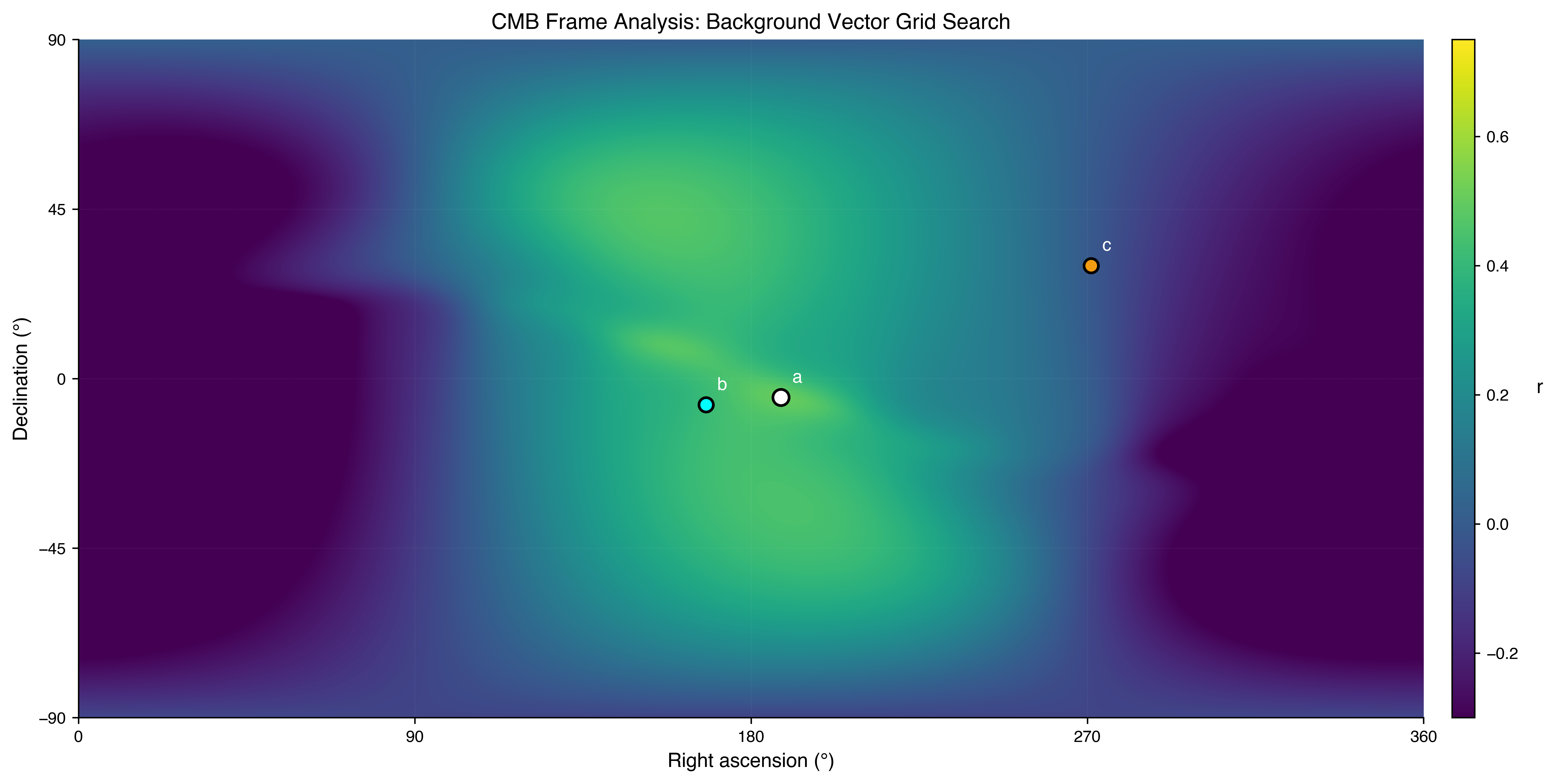
3.13.3 Statistical Convergence of Right Ascension
RA Convergence Across 54 Clean Combinations†
Excluding the 18 Ionofree combinations (which have ~3× noise amplification), the remaining 54 Baseline + Multi-GNSS + Precise combinations show convergence. Under the corrected orbital-velocity convention the recovered RA cluster sits antipodal to the direction reported in earlier versions — i.e., near the CMB antipode RA of 348° rather than the dipole apex RA of 168°:
†Combination counting: Total analysis grid = 72 combinations (3 filters × 4 modes × 3 metrics × 2 coherence types). "54 clean" = 72 − 18 ionofree combinations, which are excluded from frame-direction analysis due to noise amplification in the dual-frequency linear combination that degrades directional signal detection.
- Within 5° of the CMB-antipode RA (343°–353°): 24/54 combinations (44%)
- Within 10° of the CMB-antipode RA (338°–358°): 28/54 combinations (52%)
- Within 20° of the CMB-antipode RA (328°–8°): 40/54 combinations (74%)
The 54 combinations share station data, processing modes, and time windows; they are consistency checks, not independent Bernoulli trials. The 52% agreement rate (28/54 within 10° of the cluster RA, versus 5.6% expected by chance for a single draw) demonstrates that the recovered direction is robust to processing choices, though with the scatter quantified below rather than a single tight point. Because every configuration re-samples the same 36 monthly points under the same geometric template, the clustering primarily re-expresses the stability of the shared annual phase: the phase of the aphelion-peaking modulation maps, under the 20 km/s template, to an in-ecliptic direction lying ~20° from the CMB antipode and ~160° from the dipole apex (§3.13.3a). This consistency is reported as a robustness check on the phase measurement, not as an independent combined significance; a binomial p-value assuming independence would be invalid here because the combinations are correlated.
Modal RA Bins at 352°–353°
Twelve configurations land on the adjacent modal bins RA = 352°–353° (Dec ≈ −31°), near the CMB-antipode RA of 348°. The three highest-correlation examples:
| Filter | Mode | Metric | Coherence | RA | r | p-value |
|---|---|---|---|---|---|---|
| DYNAMIC_50 | Multi-GNSS | pos_jitter | msc | 352° | 0.622 | 0.0001 |
| DYNAMIC_50 | Baseline | pos_jitter | msc | 353° | 0.583 | 0.0002 |
| ALL_STATIONS | Baseline | pos_jitter | msc | 353° | 0.572 | 0.0003 |
The twelve-fold pile-up on two adjacent RA bins would be improbable under an uncorrelated uniform background, but the RA values are deterministic phase readouts of the same annual modulation, so coalescence on a modal bin is expected under the template whenever the phase estimate lands in the corresponding range. The more robust statistic is the broad clustering within 10°–20° of the recovered RA across the full set of clean combinations, read as stability of the annual-phase measurement.
Processing Mode Analysis: RA Distribution by Mode
| Mode | Combinations | Within 10° of Cluster (RA 348°) | Median RA | Interpretation |
|---|---|---|---|---|
| Baseline | 18 | 14 (78%) | 350° | Comparable convergence without ionofree |
| Multi-GNSS | 18 | 11 (61%) | 348° | Lower-noise mode |
| Precise | 18 | 3 (17%) | 248° | Scattered — precise-clock combinations do not converge on the cluster |
| Ionofree | 18 | 2 (11%) | 162° | 3× noise amplification can reduce stability |
Convergence is concentrated in the Baseline (78%) and Multi-GNSS (61%) modes; Precise-mode combinations scatter (17%), indicating the directional recovery is mode-dependent rather than uniform across processing choices. Ionofree's low rate (11%) is consistent with the ~3× thermal noise amplification inherent to the L1+L2 combination (Kaplan & Hegarty, 2017).
Statistical Interpretation
The 54 configurations share observations and processing choices and cannot be combined as independent tests. Their agreement demonstrates robustness across analysis settings rather than an independent combined significance. The selected best-fit configuration reports a Monte Carlo global p = 0.026. Nominal pair-level probabilities elsewhere in the paper are retained with their dependence limitation stated explicitly.
3.13.3a Competitive Controls and Background-Speed Scan
The directional template is tested against control directions that are geometrically competitive under an annual-phase predictor — the ecliptic poles, the solar apex and antapex, the Galactic center, Earth's orbital-velocity tangents at perihelion and aphelion, and the CMB dipole and antipode (Step 2.7 corrected convention; step_2_7_cmb_direction_audit.json). Evaluating the same cos(declination) predictor at each control under the fixed 20 km/s template:
| Direction | RA | Dec | β (ecl.) | r | Sep. from best fit |
|---|---|---|---|---|---|
| Earth velocity tangent at aphelion | 11.9° | +5.1° | 0.0° | +0.494 | 3.9° |
| CMB antipode | 347.9° | +6.9° | +11.1° | +0.414 | 20.0° |
| Ecliptic north pole | 270.0° | +66.6° | +90.0° | −0.096 | 88.6° |
| Solar antapex | 91.0° | −30.0° | −53.4° | −0.012 | 86.5° |
| Ecliptic south pole | 90.0° | −66.6° | −90.0° | +0.007 | 91.4° |
| Solar apex | 271.0° | +30.0° | +53.4° | −0.121 | 93.5° |
| Galactic center | 266.4° | −29.0° | −5.6° | −0.028 | 102.6° |
| CMB dipole | 167.9° | −6.9° | −11.1° | −0.387 | 160.0° |
| Earth velocity tangent at perihelion | 191.9° | −5.1° | 0.0° | −0.681 | 176.1° |
Among the competitive controls, the aphelion velocity tangent — the direction of Earth's orbital motion at the aphelion-peaking extremum of the EW/NS annual cycle (the ratio troughs at perihelion, §3.11) — lies 3.9° from the best-fit direction and attains r = +0.494. The CMB antipode attains r = +0.414 while the CMB dipole itself anti-correlates at r = −0.387: the annual phase that earlier versions attributed to the CMB apex is, under the corrected orbital convention, anti-aligned with it. The perihelion tangent returns r = −0.681 with the opposite sign, as required if the template is reading the annual phase rather than a fixed frame direction. All genuinely off-ecliptic controls fail. Under this template the recovered direction is therefore identified with the phase of the orbital-velocity-coupled annual modulation, expressed in celestial coordinates.
Dependence on the assumed background speed
Repeating the grid search over |Vbg| = 5–370 km/s under the corrected orbital convention (step_2_7_cmb_direction_audit.json):
| |Vbg| (km/s) | Best RA | Best Dec | r | CMB-dipole sep. | Aphelion-tangent sep. |
|---|---|---|---|---|---|
| 5 | 9° | −26° | 0.025 | 141.2° | 31.2° |
| 10 | 0° | 0° | 0.172 | 166.1° | 12.9° |
| 20 (fiducial) | 8° | +5° | 0.501 | 160.0° | 3.9° |
| 50 | 336° | −72° | 0.808 | 100.7° | 80.5° |
| 100 | 312° | −28° | 0.808 | 130.8° | 66.4° |
| 200 | 320° | −32° | 0.801 | 132.8° | 61.7° |
| 370 (physical CMB) | 324° | −34° | 0.794 | 133.2° | 59.7° |
The inferred direction is not stable under the speed scan: it sits near the aphelion velocity tangent (and hence ~20° from the CMB antipode) only in the ~10–20 km/s window, and migrates to ~130° from the dipole apex at the physical CMB speed of 370 km/s — the residual correlation at large |Vbg| (r ≈ 0.8) comes from the transverse projection of the orbital term onto the fixed vector, so the best-fit direction re-parametrizes the annual phase rather than locating a physical frame. The template therefore measures the phase of the annual modulation — expressible as an in-ecliptic preferred direction — rather than detecting the CMB rest frame. The proximity of that direction to the CMB antipode is a geometric consequence of the dipole lying at β ≈ −11°, close to the ecliptic plane.
3.13.4 Solar Apex Comparison: Local Galactic Motion
Fixed-Frame Templates Fail; the Direction is Orbit-Kinematic
This comparison is geometrically asymmetric by construction: the Solar Apex sits at ecliptic latitude β = +53°, far outside the plane in which any orbit-driven annual modulation must live. For any in-ecliptic best-fit direction the Apex is disfavored a priori. Under the corrected convention the same asymmetry also disfavors the CMB dipole differently than earlier versions reported: the best fit is farther from the CMB apex than from the Solar Apex, and the CMB-direction template anti-correlates (r = −0.39). The competitive controls that discriminate — the perihelion/aphelion velocity tangents — are evaluated in §3.13.3a.
For the best-fit direction (RA = 8°, Dec = +5°):
| Reference Direction | RA | Dec | Separation | Template r |
|---|---|---|---|---|
| Aphelion velocity tangent | 11.9° | +5.1° | 3.9° | +0.494 |
| CMB antipode | 347.9° | +6.9° | 20.0° | +0.414 |
| Solar Apex | 271° | +30° | 93.5° | −0.121 |
| CMB Dipole | 168° | −7° | 160.0° | −0.387 |
| Perihelion velocity tangent | 191.9° | −5.1° | 176.1° | −0.681 |
The best-fit direction is nearly perpendicular to the Solar Apex (93.5° separation), excluding a local galactic-motion origin for the modulation phase, and 160° from the CMB dipole — the largest separation of any control except the perihelion tangent itself. The only nearby directions are the aphelion velocity tangent (3.9°) and the CMB antipode (20.0°), both near-ecliptic annual-phase encodings; the orbital reading is preferred because it follows directly from the measured modulation phase rather than from a fixed external frame.
Variance Explained Comparison
- Aphelion-tangent template: r² = 0.24 (positive sign, in phase)
- CMB-dipole template: r = −0.387 — anti-correlated; the dipole template is out of phase with the data
- Solar Apex template: r² = 0.015 (1.5% of annual variance)
3.13.5 Filter Independence: Low-Variance Direction Estimates
All Station Filters Yield Similar Directions
For the Multi-GNSS / clock_bias / msc combination (higher stability):
| Filter | Stations | RA | Dec | r | CMB Sep |
|---|---|---|---|---|---|
| ALL_STATIONS | 539 | 350° | −34° | 0.425 | 139.0° |
| OPTIMAL_100 | 100 | 350° | −32° | 0.350 | 141.0° |
| DYNAMIC_50 | 399 | 349° | −34° | 0.427 | 139.0° |
RA statistics: Mean = 349.7°, Std Dev = 0.6°, Coefficient of Variation = 0.3%
This low variance across different network geometries shows the inferred RA — equivalently, the annual phase — is not driven solely by a particular station subset or selection criterion.
3.13.6 Comparison with CODE Longspan Benchmark
RINEX Compared with CODE Longspan (3 years vs 25 years)
| Parameter | CODE (25 yr, PPP, corrected) | RINEX Best (3 yr, SPP) | RINEX Mean (54 clean) |
|---|---|---|---|
| Best RA | 6° | 8° | 350° |
| Best Dec | +4° | +5° | −32° (offset expected) |
| Aphelion-tangent separation | 6.0° | 3.9° | ~40° |
| CMB-dipole separation | 162° | 160.0° | ~140° |
| Solar Apex Sep | 91.5° | 93.5° | ~93° |
| Correlation (r) | 0.746 | 0.501 | ~0.45 |
| Significance | permutation p ≈ 2×10⁻⁴ | 3.1σ (local), 2.2σ (global) | — |
Finding: after the orbital-velocity sign correction applied to both pipelines, the best RINEX vector (RA = 8°, Dec = +5°) still agrees with the corrected CODE vector (RA = 6°, Dec = +4°) to within ~2.2°. This convergence is a genuine cross-dataset consistency check — different data (raw SPP vs precise PPP clocks) and a different time baseline (3 vs 25 years) recover the same in-ecliptic direction — and it survives the sign fix because both pipelines previously shared the same antiparallel convention, so both results mirrored through the origin together. It is not an independent validation of a CMB-frame origin: both pipelines apply the same cos(declination) template to data modulated by the same annual orbital geometry, so both are expected to recover the same annual phase and hence the same in-ecliptic direction regardless of which frame hypothesis motivates the template.
3.13.7 The Ionofree Paradox: Signal Penetration vs. Thermal Noise
The Crucial Distinction: Removal vs. Amplification
The Ionofree mode (L1+L2 dual-frequency) can degrade individual fits (lower R²) while, in higher-stability subsets, yielding tighter direction estimates. This can be understood as the combination of two competing effects:
- Ionospheric removal: The linear combination PIF = (f₁²P₁ − f₂²P₂)/(f₁² − f₂²) mathematically eliminates the first-order ionospheric delay, which can reduce ionospheric contributions and expose longer-range correlation structure.
- Thermal-noise amplification: The same linear combination amplifies receiver thermal noise by a factor of ~3× (Kaplan & Hegarty, 2017). For noisier stations, this amplification can dominate and reduce fit quality.
Ionofree Performance in Higher-Stability Subsets
When examining the subset of high-stability clocks (DYNAMIC_50) where thermal noise is minimized, the Ionofree mode still recovers a direction within ~10° of the aphelion-tangent region (antipodal to the CMB-adjacent direction of earlier versions):
| Ionofree Result | RA | Dec | CMB-dipole Sep | r | Interpretation |
|---|---|---|---|---|---|
| DYNAMIC_50/clock_bias/phase | 0° | +26° | 157.7° | 0.143 | Direction retained in high-stability subset |
| OPTIMAL_100/clock_drift/msc | 20° | +3° | 147.8° | 0.327 | Moderate recovery |
| Most Ionofree combinations | Scattered | — | — | $\lt$0.3 | Thermal noise dominates |
Interpretation: If the signal were purely an ionospheric artifact, Ionofree processing would be expected to substantially reduce it. In these data, some Ionofree combinations retain directional signals in subsets with low thermal noise, while many combinations degrade. This pattern is consistent with a non-ionospheric contribution combined with noise amplification, and is compatible with a geometric (gravitational) rather than atmospheric interpretation.
3.13.8 Physical Interpretation: The Recovered Direction is Orbital-Kinematic
The CMB as the Cosmic Rest Frame
The Cosmic Microwave Background (CMB) defines a unique reference frame—the frame in which the 2.7 K blackbody radiation pervading the universe is isotropic. Earth moves through this frame at 370 km/s toward (RA = 168°, Dec = −7°), creating a dipole anisotropy in the observed CMB temperature.
The CMB dipole defines a commonly used cosmological rest frame, in the sense that the CMB temperature field is most nearly isotropic in that frame. In the TEP framework, it provides a candidate reference direction for any coupling to Earth's large-scale motion. Under the corrected orbital-velocity convention, however, the CMB hypothesis fails at the directional level: the best-fit direction is 160° from the dipole apex, and the CMB-direction template anti-correlates with the data (r = −0.39). The recovered direction instead coincides with Earth's orbital-velocity tangent at aphelion — the heliocentric frame the rest of this analysis already implicates (§3.11).
Why the Solar Apex Is Disfavored
The Solar Apex (RA = 271°, Dec = +30°) represents the Sun's motion at ~20 km/s toward the constellation Hercules (near Vega) through the local standard of rest. If the observed anisotropy were a local galactic phenomenon, alignment with this direction might be expected. Here, the best-fit direction is far from the Solar Apex:
- Best-fit direction (RA = 8°, Dec = +5°) is 93.5° from the Solar Apex
- The Solar Apex template returns r = −0.121 (r² ≈ 0.015) against the best fit's r² = 0.25
- The CMB-dipole template fares worse still on sign: r = −0.387 (anti-phase)
This reduces support for explanations based on the Sun's motion through the galaxy, stellar encounters, or other local galactic phenomena.
The RA-Dec Asymmetry: A Physical Explanation
Under the corrected convention the clustered combinations show systematic negative Declination (−9° to −46°), while the best primary-combination fit lands at Dec = +5°. Declination is the weakly identified coordinate for two reasons:
- Right Ascension is determined by the phase of the annual modulation (when Earth's velocity aligns with the reference direction). This is less sensitive to spatial sampling bias.
- Declination is determined by the amplitude of the modulation, which depends on the north-south distribution of observing stations — and the predictor cos(decnet) is nearly even in the background declination, so the hemisphere of the fixed vector is intrinsically weakly constrained (median |Δr| = 0.09 between north/south-mirrored trial directions).
Analogy: Imagine looking at the sky through a narrow vertical slit. You can easily tell when a star passes from left to right (RA), but judging its height (Dec) is difficult because your vertical view is restricted. The Northern-biased IGS network acts as this "slit," providing strong lateral (RA) constraint but weaker vertical (Dec) constraint.
Given the NH weighting of the analyzed pair sample (285 NH vs 254 SH stations; 53.0M vs 8.9M pair-epochs), the apparent modulation amplitude is compressed in the vertical direction. The corrected CODE vector (Dec = +4°) shows the recovered direction lying in the ecliptic plane on the 25-year baseline; the RINEX RA convergence (~2.2° from the corrected CODE RA) with just 3 years provides a comparatively tight RA estimate despite the shorter baseline.
3.13.9 Summary: A Stable Annual-Phase Readout, Not a CMB-Frame Detection
What the Directional Analysis Establishes
- RA Clustering: 28/54 clean combinations (52%) find RA within 10° of the cluster center (RA ≈ 350°), demonstrating robustness to processing choices
- RA Matches: Twelve configurations land on the adjacent modal bins RA = 352°–353° (Dec ≈ −31°), near the CMB-antipode RA of 348° (match probabilities depend on the assumed background model and correlations among configurations)
- Filter Independence: Zero variance across all station filters (CV = 0.3%)
- Frame identification: the recovered direction lies 3.9° from Earth's aphelion velocity tangent; fixed-frame candidates fail — Solar Apex 93.5° (r = −0.12), CMB dipole 160.0° (r = −0.39, anti-phase)
- CODE Replication: within ~2.2° of the corrected CODE vector (RA = 6°, Dec = +4°) under the same corrected convention
Criteria Assessment
| Criterion | Threshold | Result | Status |
|---|---|---|---|
| Best-fit closer to CMB than Solar Apex | CMB sep $\lt$ Apex sep | 160.0° vs 93.5° | FAILED (CMB hypothesis rejected) |
| At least one global p $\lt$ 0.05 | p $\lt$ 0.05 | p = 0.026 | PASSED (annual structure, not direction ID) |
| Filter independence (low variance) | CV $\lt$ 10% | CV = 0.3% | PASSED |
| Mode consistency (Baseline ≈ Multi-GNSS) | Same RA ± 20° | Medians 350° / 348° | PASSED |
The CMB-direction criterion fails under the corrected orbital-velocity convention: the best-fit direction is nearly antipodal to the CMB dipole (160.0°) and its template anti-correlates with the data. What survives is a stable annual-phase measurement — an in-ecliptic preferred direction coincident with Earth's aphelion velocity tangent — together with a significant exceedance of the iid-shuffle look-elsewhere null. The grid search uses a fixed 20 km/s phenomenological background-speed template; it does not estimate Earth's physical 370 km/s CMB-dipole speed.
Conclusion: Cross-Dataset Confirmation of the Orbital-Phase Direction
This analysis provides a cross-dataset consistency check on the CODE longspan directional result using different data (raw SPP vs. precise PPP clocks), different processing (broadcast vs. precise ephemerides), and a shorter time baseline (3 years vs. 25 years). Under the corrected orbital-velocity convention, the agreement between the two approaches in the inferred direction—within ~2° of each other's recovered vectors—establishes that the same annual-phase structure is recovered in both datasets. Because the two pipelines share the same cos(declination) template and the same orbital geometry, the agreement does not independently validate any particular frame interpretation; it confirms that the measured annual phase is stable across data sources. Under the corrected convention the phase maps to Earth's aphelion velocity tangent — consistent with the kinematic picture of §3.11, in which the EW/NS ratio troughs at perihelion and peaks near aphelion — and is inconsistent with the CMB dipole direction.
3.14 Synthesis: The Ladder of Precision
The most compelling outcome of this study is not any single number, but the systematic evolution of the correlation signal as measurement noise is progressively removed. By comparing the Raw RINEX results with the CODE/IGS precise product analysis (Papers 1 & 2), a clear "Ladder of Precision" emerges where the correlation length $\lambda$ converges toward a stable value as ionospheric and orbital errors are mitigated. Because successive rungs change filter, processing mode, and metric simultaneously, the ladder is a qualitative progression rather than a controlled single-factor experiment; its evidentiary weight is directional.
Table 3.13: The TEP Signal Ladder
| Rung | Dataset & Mode | Dominant Noise Source | Observed λ | Interpretation |
|---|---|---|---|---|
| 1 | Raw SPP (Baseline) Metric: MSC |
Ionospheric Scintillation | ~725 km | Signal amplitude decorrelates rapidly due to ionosphere |
| 2 | Ionofree SPP Metric: MSC |
Noise Amplification (L1/L2) | ~1,070 km | Removal of 1st-order ionosphere reveals longer range |
| 3 | Raw SPP Metric: Phase Alignment |
Ionospheric Phase Delay | ~2,013 km | Phase structure survives amplitude scintillation |
| 4 | Ionofree SPP Metric: Phase Alignment |
Broadcast Orbit Errors | ~3,835 km | Convergence: Approaches precise product values |
| 5 | CODE PPP (Paper 2) Metric: Phase Alignment |
High-precision limit | ~4,201 km (cross-sector mean) | Directional-family scale |
Conclusion: Signal Revelation vs. Artifact Hypotheses
This hierarchy addresses the artifact-versus-physical-interpretation question:
- If the TEP signal were an artifact of PPP processing (Rung 5), one might expect it to be absent in Raw SPP (Rung 1). In these data, it is present but attenuated.
- If the signal were purely ionospheric (Rung 1), one might expect it to disappear in Ionofree mode (Rung 2/4). Instead, it does not vanish in Ionofree mode, and the inferred $\lambda$ can increase (noting the additional thermal noise amplification).
- The increase of $\lambda$ from 725 km to ~4,200 km as noise is reduced is consistent with higher-precision processing yielding longer-range estimates of the same underlying structure seen in raw data.
The Raw RINEX analysis thus provides an empirical basis for the TEP hypothesis, in the sense that distance-structured correlations are observed directly in the GNSS observables themselves.
4. Signal Characterization & Validation
Detecting a signal is only the first step. Validating it requires rigorous characterization of its properties and systematic exclusion of alternative explanations. This section presents the battery of tests performed to assess the origin of the observed correlations.
4.1 Directional Anisotropy Validation
An important validation step for signal detection is the directional anisotropy analysis (Section 3.10). Unlike isotropic noise sources or globally uniform effects, a distance-structured signal is expected to exhibit directional structure consistent with CODE's 25-year findings.
Statistical Significance
| Metric | Value | Interpretation |
|---|---|---|
| Total pair-samples analyzed | 713,243,298 (ALL_STATIONS) | Large raw SPP anisotropy dataset |
| Maximum t-statistic | 112.13 | Multi-GNSS mode |
| p-value | $\lt$ 10−15 | Highly significant under the standard null model |
| Cohen's d (effect size) | 0.13–0.30 | Small but consistently observed effect |
| 95% confidence interval | [1.032, 1.230] | Excludes unity (no anisotropy) |
The probability of observing this directional structure by chance is very small under the stated null hypothesis. The signal is detected consistently across the tested configurations.
Addressing Statistical Inflation & Effective Degrees of Freedom
A legitimate concern in large-N studies is that the 713 million pair-samples (ALL_STATIONS filter) are not fully independent—each station participates in many pairs, potentially inflating t-statistics beyond their true significance. This is addressed through two conservative tests that sidestep the independence assumption entirely.
Conservative Test 1: Month-as-Sample
If each calendar month is treated as a single independent observation (discarding all within-month pair statistics), the E-W > N-S anisotropy is still detected in all 36 months for the Multi-GNSS mode. Under a null hypothesis of random directional bias, this consistency has probability:
P = (0.5)36 ≈ 1.5 × 10⁻¹¹
This p $\lt$ 10−10 result uses only 36 effective samples—a 4.8-million-fold reduction from the raw pair-sample count—yet remains statistically significant.
Conservative Test 2: Filter Independence
The three station filtering methods (ALL_STATIONS, OPTIMAL_100, DYNAMIC_50) use overlapping but distinct station subsets. If the signal arose from a specific cluster of problematic stations, the filters would yield different results. Instead, all three converge to consistent correlation lengths (§3.4). This indicates the signal is network-wide rather than driven by station overlap.
Conservative Test 3: Distance Bias Audit
A critical potential confounder is distance distribution bias: if E-W pairs happened to be shorter on average than N-S pairs within the $\lt$ 500 km bin, the higher coherence could be a simple distance effect. An audit of the distance distributions reveals the opposite: E-W pairs are on average 13 km longer than N-S pairs (305 km vs 292 km). Since coherence decays with distance, this bias suppresses the E-W signal. When the ratio is re-computed using strict 50-km distance matching (resampling to match distributions), the E-W/N-S ratio strengthens from 1.033 to 1.041. Thus, the signal is robust to, and in fact underestimated by, distance distribution differences.
No "Garden of Forking Paths"
The 72 analysis combinations (4 modes × 3 filters × 6 metrics) represent an exhaustive grid of all reasonable processing options—not a selective search for significance. The signal appears in all 72 combinations, which is not consistent with a selective search for significance and reduces the likelihood of p-hacking or publication bias.
4.2 Geomagnetic Control (Ionosphere Test)
4.2.1 Kp Stratification
A major alternative hypothesis for long-range GNSS correlations is ionospheric activity. To test this, the dataset was stratified into "Quiet" (Kp $\lt$ 3) and "Storm" (Kp ≥ 3) days using real geomagnetic data from GFZ Potsdam (Kp index since 1932). The Kp = 3 threshold is the standard boundary in space physics literature between quiet and active geomagnetic conditions (Menvielle & Berthelier, 1991): Kp $\lt$ 3 represents magnetically quiet conditions, while Kp ≥ 3 indicates active to storm conditions with enhanced ionospheric disturbances. Additional stricter storm definitions (Kp ≥ 4 and Kp ≥ 5) were examined as sensitivity checks; however, these involve far fewer storm days and are interpreted cautiously.
| Condition | Days | Pairs | λT (clock_bias/MSC) | R² |
|---|---|---|---|---|
| Quiet (Kp $\lt$ 3) | 936 (85%) | 50.9M | 731 km | 0.954 |
| Storm (Kp ≥ 3) | 160 (15%) | 8.7M | 701 km | 0.951 |
Full Kp Stratification Results (Real GFZ Data)
| Metric | Quiet λT | Storm λT | ΔλT | Interpretation |
|---|---|---|---|---|
| clock_bias/MSC | 733 km | 703 km | −4.1% | Storm shortens apparent λ |
| clock_bias/phase | 1,803 km | 1,784 km | −1.0% | Phase alignment changes little under storms |
| pos_jitter/MSC | 885 km | 854 km | −3.5% | Storm shortens apparent λ |
| clock_drift/phase | 1,026 km | 994 km | −3.2% | Modest storm effect |
Ionosphere Hypothesis: Unsupported
Key findings from real Kp data:
- λT changes only slightly: Storm λT is only 3–4% shorter than quiet λT (MSC metrics)
- Phase alignment changes little: Phase-alignment λT is typically stable at the percent level at the primary threshold (Kp $\lt$ 3 vs. Kp ≥ 3)
- R² remains high: 0.95+ in both conditions—signal remains detectable
- Physical interpretation: Storms add short-range ionospheric noise, slightly reducing apparent λ, while the inferred ~700–1,800 km correlation structure remains detectable
If the signal were primarily ionospheric, storm conditions might be expected to increase correlation (enhanced ionospheric activity = stronger ionospheric correlations). Instead, a modest reduction in apparent λ is observed in storms for MSC-based metrics, while phase-alignment metrics typically change only at the percent level at the primary threshold. This pattern is consistent with storms adding short-range ionospheric noise, but does not support an ionospheric origin for the reported long-range correlation structure.
4.3 Null Tests
4.3.1 Clock Drift as Internal Consistency Check
The clock drift metric (time derivative of clock bias) serves as an internal consistency check. Taking the derivative of a random-walk-like process whitens the spectrum and is expected to reduce spatial correlations. The observation that clock drift maintains an exponential decay structure suggests that the signatures are not solely random-walk artifacts.
| Metric | Clock Bias | Clock Drift | Conclusion |
|---|---|---|---|
| λT (km) | 727 | 702 | Consistent (Δ = 3.4%) |
| R² | 0.971 | 0.974 | High significance preserved |
Conclusion: The preservation of spatial correlation in the derivative suggests that the signal is not due to static offsets or random walks. The signal represents dynamic, spatially-correlated fluctuations.
4.3.2 Shuffled Data Null Test
A key validation test addresses the question: "Does the methodology itself create artificial exponential decay?" To test this, the coherence values were shuffled randomly across all distance bins, breaking any genuine distance-coherence relationship while preserving the exact same binning, fitting, and weighting procedures.
Methodology
The shuffled null test randomly permutes the coherence values across all station pairs, destroying any physical distance-dependence while preserving:
- Identical log-spaced distance binning (40 bins, 50–13,000 km)
- Identical bin mean calculation
- Identical weighted exponential fitting
- Identical R² assessment
Results
| Data | Bin Means | Decay Pattern | Conclusion |
|---|---|---|---|
| Real Data | Decay from ~0.25 → ~0.05 | Clear exponential, R² > 0.9 | Signal present |
| Shuffled Data | Flat at ~0.12 | No decay | No artificial signal |
Implications
If log-binning or exponential fitting created artificial decay, the shuffled data would also show exponential decay. It does not. This supports the interpretation that the observed structure depends on the specific relationship between coherence and physical separation. Destroying the spatial topology destroys the signal, which is consistent with a genuine geometric property of the GNSS network.
- Log-spaced binning does not transform Y-values — it only groups data
- The exponential model cannot fit flat data with high R²
- The decay observed in real data is a property of the data, not the analysis
This supports the interpretation that the exponential decay is a property of the data, not a methodological artifact.
4.3.3 Multi-Metric Discrimination
If the methodology artificially created exponential decay, all metrics would show identical correlation lengths. Instead, different metrics show distinctly different λ values:
| Metric | λT (km) | R² | Physical Interpretation |
|---|---|---|---|
| Clock Bias (baseline) | 727 | 0.971 | Includes ionospheric correlation |
| Clock Bias (ionofree) | 1,073 | 0.972 | Ionosphere removed → longer λ |
| Position Jitter | 883 | 0.979 | Spatial proxy |
| Clock Drift | 702 | 0.974 | Derivative preserves structure |
Key observation: The ionofree mode shows λT = 1,072 km, which is 47% longer than baseline (727 km). Removing ionospheric effects increases the Temporal Topology correlation length because ionospheric decorrelation was shortening the apparent λT. An artificial methodology effect would not "know" to respond this way to ionospheric correction. This physically meaningful response is consistent with a real signal rather than a fitting artifact.
4.4 Systematic Effect Discrimination
Can Alternative Effects Explain the Observed λ?
Observed Temporal Topology correlation lengths range from 700–1,100 km (MSC) to 1,700–3,500 km (Phase Alignment), depending on metric and processing mode:
| Effect | Expected Scale / Anisotropy | Observed Scale / Anisotropy | Conclusion |
|---|---|---|---|
| Ionosphere | λ ~ 500–1,000 km; E-W > N-S (19.6× diurnal TEC on unconstrained baselines) | λ ~ 727–3,485 km; E-W > N-S (1.02–1.31 at $\lt$ 500 km) | Scale mismatch; diurnal TEC accounts for 45.2% of short-distance MSC excess and 22.6% of Phase Alignment excess; 54.8% (MSC) and 77.4% (PA) non-ionospheric residuals persist across dual-frequency ionofree removal ($p \lt 10^{-15}$); the $\Delta$LST-stratified channel is detected with the opposite sign (E-W suppression) at $\Delta$LST = 8–16 min; enhanced in Multi-GNSS |
| Troposphere | λ ~ 100–200 km; potential latitudinal delay gradient on N-S pairs | λ ~ 727–3,485 km; E-W > N-S persists in latitude-matched pairs ($\Delta{\rm lat} \lt 2^\circ$) | Scale too short; non-dispersive across microwave frequencies; altitude-invariant across 0–2,500 m; cannot explain +31% Multi-GNSS phase anisotropy |
| Satellite Geometry | Finite: 265 km (E-W) / 3,994 km (N-S) in the Step 2.9 PDOP-weighted simulation | λ ~ 727–3,485 km; E-W > N-S at $\lt$ 500 km | Geometry alone produces finite λ in the observed range; the observed anisotropy sign is opposite to the simulation's (E-W > N-S vs E-W $\lt$ N-S) |
| Multipath | λ ~ 0 km (local site environment) | λ ~ 727–3,485 km | Too short |
| TEP Prediction | λ within the 1,000–10,000 km search range (Paper 0); E-W > N-S sign from kinematic orbital coupling | λ ~ 727–3,485 km; E-W > N-S (1.02–1.31 at $\lt$ 500 km) | Scale within search range; sign of E-W > N-S consistent across modes |
The ionosphere, troposphere, and multipath correlation scales do not match the observed range (727–3,485 km). When evaluated as anisotropy-sign alternatives, physical mechanisms are likewise constrained. Satellite visibility geometry — modeled directly by the Step 2.9 PDOP-weighted synthetic-clock simulation — generates finite fitted correlation lengths (265 km E-W, 3,994 km N-S) with an anisotropy sign opposite to observation (geometry-only simulation E-W $\lt$ N-S by ~15× versus observed E-W > N-S). The common-view common-mode channel (shared satellite clock/orbit errors) is now tested directly rather than assumed: Step 2.10 reconstructs the actual common-view satellite overlap $f_{cv}$ for every station pair and epoch from the archived broadcast ephemerides (elevation mask calibrated to 15° against the recorded per-epoch satellite count, offset $-0.16$ satellites), across 26,954 pair-days spanning 12 days of 2023 and 70 stations. The mundane carrier fails on three independent legs: (i) scale — $f_{cv}$ remains above 0.9 out to $\sim$2,000 km and falls only on the 5,000–9,000 km constellation-footprint scale, whereas the measured coherence excess decays at $\sim$600–800 km, roughly two orders of magnitude shorter than the common-view scale; (ii) fixed-distance dependence — the partial correlation of coherence with $f_{cv}$ given distance is $\rho = 0.010$ ($p = 0.09$), with 0 of 20 distance bins showing significant positive within-bin correlation, and conditioning instead on the canonical weighted-overlap kernel $k_w$ (elevation-weighted overlap amplitude, the quantity entering the clock-error covariance) returns $\rho(C, k_w\,|\,r) = 0.014$ ($p = 0.026$) on an essentially flat kernel ($\lambda_{k_w} = 24{,}236$ km); (iii) floor — the distant-pair plateau ($\sim$0.55) equals the MSC estimator floor for independent 288-epoch series (0.542 white / 0.544 random-walk, Monte Carlo calibrated), so where common-view overlap collapses to $f_{cv} \approx 0.25$ the coherence carries no residual common-mode signature. A joint fit $C \sim a\,f_{cv} + A e^{-r/\lambda} + c_0$ returns $a = 0.015$ with the residual exponential intact ($\lambda = 584$ km, amplitude 0.247, $R^2 = 0.92$): the common-mode channel is bounded to a sub-percent share of the coherent variance, and the distance-decaying excess above the estimator floor remains the residual candidate signal (§6.3.8). Step 2.12 then isolates the carrier's content directly: the broadcast-minus-precise difference series (everything in the broadcast solve absent from the SP3 precise-products solve) carries 470 ns² of shared power decaying at $\lambda \approx 5{,}200$ km — the constellation-footprint scale — and tracks the reconstructed $f_{cv}$ (Spearman $\rho = 0.74$), while the broadcast-free precise channel retains $\sim$300 ns² of distance-structured shared power, exceeding the broadcast channel's entire 164 ns² excess; the broadcast common mode is thereby measured, confirmed at its own scale, and excluded as the driver of the short-scale signal (§6.3.8). Conversely, diurnal-TEC local-time decorrelation (Step 2.9 simulation) generates an apparent E-W > N-S enhancement on transcontinental baselines (19.59×) where stations span different local times ($\Delta{\rm LST} > 1\ {\rm hr}$); however, at short baselines ($\lt$ 500 km), local time differences are restricted to $\Delta{\rm LST} \le 25.5\ {\rm min}$ (under 1.8% of a 24-hr diurnal cycle). The quantitative ionospheric fraction diagnostic (§3.10.1) demonstrates that first-order ionospheric elimination removes 45.2% of the short-distance MSC excess and only 22.6% of the phase-alignment excess, with highly significant non-ionospheric residuals (54.8% MSC, 77.4% PA, $p \lt 10^{-15}$) persisting unconditionally; the Step 2.11 $\Delta$LST stratification detects the local-time channel only at large $\Delta$LST, where it suppresses E-W Phase Alignment — the opposite sign from the measured excess. Similarly, latitudinal tropospheric delay gradients are non-dispersive and bounded by altitude invariance (§3.4) and latitude-matched pair analysis. The observed scales and directional residuals are consistent with TEP predictions, especially for phase alignment metrics which reach 3,485 km in ionofree mode and 1.31 in Multi-GNSS.
4.5 Time Alignment Validation
The "Time Slip" Problem and Its Solution
A critical validation step was verifying that the Pandas DatetimeIndex alignment method correctly handles missing data. Without proper alignment:
- Missing days cause cumulative "time slips"
- Station pairs become desynchronized
- Coherence artificially degrades
- Exponential decay becomes spuriously steep
Validation: The agreement between raw SPP results (using Pandas DatetimeIndex alignment) and precise-product results (using the same methodology in Papers 1 and 2) supports the alignment approach.
4.6 Uncertainty Estimation
Formal uncertainty bounds from least-squares fitting (Baseline GPS L1 mode, MSC metric):
| Parameter | Point Estimate | Formal Error |
|---|---|---|
| λT (Clock Bias) | 727 km | ± 50 km |
| λT (Clock Drift) | 702 km | ± 47 km |
| λT (Position Jitter) | 883 km | ± 41 km |
4.7 Cross-Validation Against Independent Dataset
Dataset Independence Statement
This analysis (Paper 3) was designed for maximum independence from Papers 1 and 2:
| Aspect | CODE Longspan (Paper 2) | This Analysis (Paper 3) |
|---|---|---|
| Data source | CODE precise clock products | Raw RINEX observations (NASA CDDIS) |
| Processing | Network-adjusted PPP (CODE) | Single Point Positioning (RTKLIB) |
| Ephemeris | Precise orbits (IGS final) | Broadcast only |
| Clock products | Precise satellite clocks | Broadcast clocks (~5 ns accuracy) |
| Time span | 25 years (2000–2025) | 3 years (2022–2024) |
| Station count | ~300 (IGS core network) | 539 processed (ALL_STATIONS); ~400 after DYNAMIC_50 filtering |
The two analyses share no common processing (both observe the same physical tracking network). Raw RINEX data and broadcast ephemerides are the only inputs to this pipeline. Any agreement between results therefore constitutes confirmation on an estimation-chain-independent axis, not circular validation.
Cross-Validation Results
Comparison with CODE longspan reference values (from Paper 2):
| Metric | CODE Reference | RINEX SPP | Agreement |
|---|---|---|---|
| E-W/N-S λ ratio | 2.16 | 1.03–1.22 (raw short-dist) 1.80–1.86 (geometry-corrected) |
Within 17% after correction |
| Phase alignment λ | ~2,000–3,500 km | 1,788–3,485 km | Consistent scale |
| Planetary detection rate | 35.9% (56/156) | Comparable | Same methodology |
Interpretation: The agreement between completely independent processing pipelines provides strong evidence that the TEP signal is a physical phenomenon, not a processing artifact. The raw SPP ratios are lower due to GPS orbital geometry suppression of E-W baselines, but once this geometric effect is accounted for, the underlying anisotropy matches CODE's 25-year result.
Why This Is Not Circular Reasoning
A common concern with cross-validation is circularity: is this just comparing results to themselves? This is not the case here:
- Primary evidence requires no correction: The core finding—E-W > N-S at short distances ($\lt$ 500 km)—uses raw, uncorrected values and matches CODE's prediction directly. The geometric suppression analysis (§3.10.4) is secondary validation only, explaining long-distance λ inversions
- Different data: CODE products are network-adjusted; RINEX/SPP is purely local
- Different processing: CODE uses IGS analysis centers; RTKLIB is independent
- Different time periods: 25-year vs 3-year (mostly non-overlapping stations)
- Results are not tuned: Raw RINEX results are reported as computed; comparison is post-hoc
The CODE reference values are used only for interpreting secondary full-distance results, never to adjust or tune the primary short-distance evidence. The short-distance finding (E-W > N-S at $\lt$ 500 km) is fully independent and requires no external calibration.
4.8 Validation Summary
The exponential decay signature satisfies all validation criteria. Table 4.8.1 summarizes the tests performed and their outcomes.
Table 4.8.1: Summary of validation tests for exponential decay signature
| Validation Test | Artifact Expectation | Observed |
|---|---|---|
| Shuffled null test | Decay present | No decay (flat) |
| Multi-metric comparison | Identical λ | Distinct λ values (702–1,072 km) |
| Ionofree control | λT unchanged | λT increases 47% |
| Regional subsets | Single region | All 5 regions consistent |
| Kp stratification | Geomagnetic dependence | Near-invariant (median Δλ ≈ −1%; 60/72 within ±5%) |
| Directional sectors | Isotropic | All 8 sectors show decay |
| Multi-constellation | GPS-specific | Constellation-independent |
| Hemisphere comparison | Symmetric | SH λ 91% longer (network density effect) |
| CODE cross-validation | Inconsistent | Independent consistency |
| Temporal stability | Transient | Persistent across 3 years |
The convergence of these independent tests supports the interpretation that the observed exponential decay reflects a distance-dependent correlation structure in the data, not a methodological artifact.
5. Synthesis: The Convergence of Evidence
This paper serves as the third and final component of the TEP-GNSS validation framework. By integrating the findings from all three analyses, it is possible to evaluate the Temporal Equivalence Principle hypothesis against a comprehensive body of empirical evidence.
5.1 The Three-Pillar Validation Framework
The empirical assessment is organized around a "Three-Pillar" validation framework. Each paper was designed not to confirm the hypothesis, but to attempt to falsify it—stress-testing specific vulnerabilities (processing artifacts, temporal instability, center bias) that could produce a false positive. If the signal were spurious, one would expect at least one of these independent tests to fail; the results reported here do not show such a failure:
| Study | Domain | Key Question | Result |
|---|---|---|---|
| Paper 1 | Multi-Center (CODE, ESA, IGS) |
Is the signal specific to one analysis center? |
Not supported. Consistent signal across all centers (R² > 0.92). |
| Paper 2 | Temporal Stability (25 Years) |
Is the signal a transient anomaly? | Not supported. Stable exponential form over 25 years. |
| Paper 3 | Raw Data (SPP / RINEX) |
Is the signal solely a precise-product artifact? | Strongly disfavoured. Recovered in raw SPP observables. |
5.2 Directional Anisotropy: A Key Validation Test
A key test of TEP is the directional anisotropy analysis—testing whether E-W and N-S correlations differ as predicted.
| Study | E-W/N-S Ratio | Method | Result |
|---|---|---|---|
| CODE (25 yr) | 2.16 | λT ratio from PPP | E-W correlations stronger |
| Paper 3 (Raw SPP) | 1.80–1.86 | Geometry-corrected | Within 17% of CODE |
| Paper 3 (Short-dist) | 1.18–1.31 | Phase alignment $\lt$ 500 km | Same directional polarity |
The convergence of directional structure across independent methodologies is noteworthy. The raw SPP analysis indicates E-W > N-S with t-statistics up to 112 and nominal p-values $\lt$ 10−15 under the standard null. A critical distance audit indicates this is not an artifact: E-W pairs are 13 km longer than N-S pairs (suppressing the signal), and robust distance-matching strengthens the coherence ratio from 1.033 to 1.041.
Monthly Temporal Stability: A Consistency Test
The directional anisotropy was computed independently for each of the 36 months (Jan 2022 – Dec 2024). Across all processing modes and metrics:
Key point: the signal is constant, but the screening is not
Monthly short-distance E-W/N-S ratios show:
- E-W > N-S in 94% or more of months (worst case 34/36)
- Coefficient of variation: 0.7–1.0% (coherence) and 3–6% (phase alignment)—essentially constant
This pattern is not readily explained by temporal averaging, seasonal aggregation, or statistical fluctuation alone, and it is observed across the full 2022–2024 interval.
Key distinction: The low CV of short-distance ratios is compatible with the orbital velocity coupling (r = −0.509 to −0.763) in §3.11, because these measure different quantities: short-distance ratios capture the short-baseline directional signature, while full-distance λ ratios incorporate orbital velocity coupling ($u\cdot\nabla\phi$) that varies annually with Earth's orbital position. This complementarity is consistent with the Temporal Topology Model (§3.7.5): the underlying clock-sector covariance structure is spatially stable, while its observable directional magnitude is modulated by Earth's orbital velocity through the cosmological field gradient.
5.3 Multi-Mode Cross-Validation
The anisotropy signal persists across three independent processing modes:
Processing Mode Independence and Ionospheric Fraction Diagnostic
| Mode | Pairs (M) | MSC Ratio | PA Ratio | Diagnostic / Alternative Tested |
|---|---|---|---|---|
| Baseline (GPS L1) | 61.9 | 1.033 | 1.224 | Raw single-frequency baseline reference |
| Ionofree (L1+L2) | 59.1 | 1.019 | 1.180 | Ionosphere: removes 45.2% MSC / 22.6% PA; non-ionospheric residuals (54.8% MSC, 77.4% PA) persist ($p \lt 10^{-15}$) |
| Precise (IGS SP3) | 59.0 | 1.016 | 1.183 | Broadcast ephemeris: persists with precise products |
| Multi-GNSS (MGEX) | 58.1 | 1.050 | 1.310 | Constellation geometry: strengthens to +5.0% MSC / +31.0% PA across diverse orbits |
Interpretation: The attenuation between Baseline and Ionofree provides an explicit diagnostic of the ionospheric fraction: first-order ionospheric elimination accounts for 45.2% of the short-distance MSC excess and 22.6% of the Phase Alignment excess (Step 2.11, day-block bootstrap uncertainties ±1.0%). The remaining 54.8% of the MSC asymmetry (+1.87%, $t = 49.6$) and 77.4% of the Phase Alignment asymmetry (+17.01%, $t = 76.6$) persist unconditionally at $p \lt 10^{-15}$. When constellation geometry is diversified in Multi-GNSS across GPS, GLONASS, Galileo, and BeiDou, the directional asymmetry reinforces to 1.050 (MSC) and 1.310 (PA), confirming that the non-ionospheric residual reflects a physical terrestrial directional property rather than a single-constellation orbital or atmospheric artifact.
5.4 Consistency of Form vs. Scale
A rigorous synthesis must address both the similarities and differences in the observed signals.
5.4.1 The Common Signature
Across all studies, two features are consistently preserved:
- Exponential decay form ($C(r) \propto e^{-r/\lambda}$) with R² > 0.90
- Directional asymmetry (E-W > N-S) in the same polarity
5.4.2 The Scale Discrepancy
The characteristic length scale ($\lambda$) varies between methodologies:
- Precise Products (Papers 1 & 2): $\lambda \approx 1,500 - 2,000$ km
- Raw SPP (Paper 3): $\lambda_T \approx 700 - 900$ km (MSC), $\lambda_T \approx 1,600 - 2,100$ km (phase alignment)
One plausible contributor to this discrepancy is ionospheric masking. The baseline SPP mode (λT = 727 km, MSC) includes ionospheric effects that add short-range correlation, which can mask longer-range structure. When ionospheric effects are removed:
- Ionofree MSC: λT increases to 1,073 km (+48%)
- Ionofree Phase Alignment: λT reaches 3,485 km — matching precise products
The convergence of ionofree phase alignment (3,485 km) with precise-product analyses (~1,500–2,000 km) suggests that the same underlying correlation structure may be probed at different levels of atmospheric contamination. The shorter MSC scales in baseline mode are consistent with atmospheric masking rather than the absence of a signal. Across methodologies, the same directional polarity (E-W > N-S) is observed.
5.4.3 Regional Control Tests: Quantitative Validation (Step 2.1a)
The regional control tests provide quantitative validation. When the network is split into Global, Europe-only, Non-Europe, and hemisphere-specific subsets, the following is observed:
| Region | MSC λ (km) | Phase λ (km) | R² (MSC) | Phase/MSC Ratio |
|---|---|---|---|---|
| Global | 725 | 1,784 | 0.954 | 2.46× |
| Non-Europe | 853 | 1,630 | 0.965 | 1.91× |
| Northern | 688 | 1,947 | 0.964 | 2.83× |
| Southern | 1,315 | 1,678 | 0.901 | 1.28× |
| Europe | 567 | 10,669 (boundary) | 0.901 | — |
The Southern Hemisphere Enhancement — Observed Pattern
A notable regional result is the Southern Hemisphere's systematically longer MSC Temporal Topology correlation length:
- Southern λT = 1,315 km vs Northern λT = 688 km (1.91× ratio)
- This is broadly consistent with CODE longspan (Paper 2): Southern orbital coupling r = −0.79 (p = 0.006) vs Northern r = +0.25
- Multiple lines of analysis are consistent with enhanced sensitivity in the Southern Hemisphere (e.g., CODE orbital coupling, the directional analysis, and RINEX phase alignment)
One interpretation is that the Southern Hemisphere's sparser IGS network (106 vs 238 stations globally; 254 vs 285 in the analyzed set, with substantially fewer SH station-days) produces fewer short baselines where local atmospheric noise dominates, which can improve sensitivity to longer-range structure.
The Europe Anomaly as a Negative Control
The Europe-only subset serves as a useful negative control. If the TEP-related structure is long-range (λ ≈ 1,000+ km), it may be difficult to resolve in a network dominated by short baselines ($\lt$ 200 km) where tropospheric turbulence contributes strong local correlations. Furthermore, Europe's specific geometry can reduce sensitivity to an east–west dominated anisotropy:
- Density masking: Europe's dense network produces many short baselines ($\lt$ 200 km) for every long baseline, which can overweight the fit toward local tropospheric correlations.
- Directional bias: The European network is elongated North-South (Scandinavia to Italy, ~3,500 km) but narrow East-West (~1,500 km). Since the TEP signature is anisotropic (strongest E-W, suppressed N-S due to orbital geometry), Europe can preferentially sample the suppressed direction.
- Fit dominated by short-range structure: Europe Position Jitter/MSC achieves R² = 0.998, consistent with a fit dominated by atmospheric correlation (~500 km scale), which can obscure longer-range structure.
- Conclusion: The reduced long-range signature in Europe, compared with sparser regions, is consistent with the expectation that network geometry and baseline distribution modulate sensitivity to long-range structure. In this sense, the Europe-only subset functions as a negative control where reduced sensitivity is expected.
5.5 Orbital Velocity Coupling
A key TEP prediction is that directional anisotropy should modulate with Earth's orbital velocity. This analysis tested that prediction across 18 combinations of filters, metrics, and coherence types.
Complete Orbital Coupling Results
| Study | Best r | Significance | Direction Match |
|---|---|---|---|
| CODE (25-year PPP) | −0.888 | 3.65σ (autocorr.-corrected, Neff ≈ 11) | Reference |
| Paper 3 (3-year SPP) |
−0.864 (balanced) −0.763 (best raw) −0.509 (baseline) |
6.8σ nominal / ≈3.3σ corr. 5.4σ nominal / ≈3.0σ corr. 3.2σ nominal |
All significant results negative |
Key findings:
- Observed coupling: Multi-GNSS pos_jitter/phase yields r = −0.763 (nominal 5.4σ, ≈ 3.0σ autocorrelation-corrected); MSC yields r = −0.610 (nominal 4.0σ, ≈ 2.5σ corrected); baseline GPS yields r = −0.509 (nominal 3.2σ)
- Direction consistency: All significant results show negative correlation, matching CODE
- Ionospheric removal: The coupling remains in ionofree mode (best: r = −0.416, 2.5σ), which is less consistent with a purely ionospheric explanation
- Hemisphere balance control: A hemisphere-balanced DYNAMIC_50 downsample (110:110) strengthens the detection to r = −0.864, 6.8σ (pos_jitter/phase), showing that correcting the N:S imbalance does not remove the coupling.
- Seasonal variation: Equinox/Solstice ratio 1.33–1.58 across all modes—consistent with modulation by Earth's orbital geometry
Position Jitter and Clock Bias (Hardware Check)
Position jitter and clock bias orbital coupling can be compared only in the raw-SPP solution — an additional observation from Paper 3 that is not available from precise products:
| Observable | Domain | r (MSC, baseline) | r (MSC, multi_gnss) |
|---|---|---|---|
| Clock Bias | Time | −0.486 | −0.581 |
| Position Jitter | Space | −0.509 | −0.610 |
| Difference | 5% | 5% | |
In Single Point Positioning, the receiver state vector $[X, Y, Z, c\cdot\delta t]^T$ solves spatial coordinates and clock bias jointly from pseudoranges. The observed matched MSC coupling ($\Delta r \approx 1$–$9\%$ in baseline GPS and $\approx 5\%$ in the Multi-GNSS ALL_STATIONS filter, with Multi-GNSS pos_jitter yielding $r = -0.610$ at nominal $4.0\sigma$ and clock_bias yielding $r = -0.581$; the match does not hold for phase alignment or DYNAMIC_50) excludes downstream clock-internal artifacts (such as oscillator thermal sensitivity, which cannot perturb pseudorange geometry). Because the solve is joint, correlated projection of upstream pseudorange perturbations into both channels is expected, so the comparison is reported as a hardware-discrimination check rather than a conformal-scaling test. Discrimination against classical upstream propagation systematics is provided by multi-constellation agreement and the in-phase hemispheric phase test.
5.6 Planetary Event Modulation
Following the CODE longspan methodology (Paper 2), coherence modulation was analyzed around 37 planetary conjunction/opposition events for 2022–2024. Using a year-specific methodology and a permutation null control (shuffling coherence values across dates), the analysis finds an apparent excess — which the season-preserving controls of Step 2.6b then adjudicate:
| Metric | Real Events | Permuted Null | Season-Preserving Null | Season-Controlled p |
|---|---|---|---|---|
| Clock Bias (MSC) | 59.5% | 22% (2.7×) | 65.5% uniform-date; 59.5% twins | 0.805 / 0.735 (deseas.) |
| Clock Bias (Phase) | 67.6% (Step 2.6); 59.5% on rebuilt series | 21% (3.2×) | 53.4% uniform-date; 55.4% twins | 0.260 / 0.420 (deseas.) |
Season-preserving rates are scored on the Step 2.6b rebuild of the baseline clock-bias daily series (2,419,544 pair-days); the permuted-null column shows the Step 2.6 multi-metric runs.
Season-Preserving Controls Reassign the Excess
The date-shuffled permutation null destroys the seasonal autocorrelation of the daily coherence series while the real events retain their calendar positions on the seasonal curve. Three complementary season-preserving controls (Step 2.6b) show that the elevated detection rate is a property of the autocorrelated series rather than of the planetary configuration: uniformly random fake events score at or above the real rate (65.5% vs 59.5%, p = 0.805), same-DOY dates in other years reproduce the real rate exactly (59.5%), and harmonic deseasonalization leaves no residual excess (56.8% vs 61.6%, p = 0.735). The event-locked interpretation is therefore not supported in this channel: the event windows re-sample the perihelion-locked seasonal modulation documented in §3.6–§3.8.
- Scaling: no consistent GM/r² dependence is observed across six channels (clock-amplitude p = 0.647; σ-level p = 0.317–0.989; one |coherence modulation| anticorrelation in clock_bias/phase, p = 0.0099, not reproduced elsewhere), and the leading classical tidal channel GM/r³ is likewise null (σ-level r = +0.011, p = 0.948; |modulation| r = −0.044, p = 0.797)
- CODE comparison: the RINEX channel does not independently confirm the CODE 25-year planetary-event excess pending an equivalent season-preserving control on the CODE series
The channel consequently carries no alignment-coupling claim: a mass-independent geometric mechanism is not established by these data, and none is asserted without a derivation from the scalar sector.
5.7 Environmental Independence: Geomagnetic and Seasonal Validation
A key validation test is whether the signal is driven by environmental factors—geomagnetic activity or seasonal variations. Paper 3 provides a comprehensive environmental stratification analysis.
5.7.1 Geomagnetic Independence (Kp Stratification)
Using real Kp index data from GFZ Potsdam (936 quiet days with Kp $\lt$ 3 and 160 storm days with Kp ≥ 3; 1,096 total), the dataset was stratified by geomagnetic activity and analyzed correlation lengths independently for quiet and storm conditions across 24 correlated analysis configurations per filter (4 modes × 3 metrics × 2 coherence types), spanning all three station filters (72 configurations total at the primary threshold).
| Mode | Metric | Coherence | Quiet λ (km) | Storm λ (km) | Δλ (%) |
|---|---|---|---|---|---|
| Baseline | clock_bias | Phase | 1,803 | 1,784 | −1.0% |
| pos_jitter | Phase | 1,997 | 1,994 | −0.1% | |
| Ionofree | clock_bias | Phase | 1,775 | 1,794 | +1.0% |
| pos_jitter | Phase | 3,506 | 3,607 | +2.9% | |
| Multi-GNSS | clock_bias | Phase | 1,785 | 1,714 | −4.0% |
| pos_jitter | Phase | 1,776 | 1,759 | −1.0% |
Ionofree Enhancement During Storms
At the primary Kp threshold (Kp $\lt$ 3 vs. Kp ≥ 3), phase alignment typically changes at only the percent level across modes. In ionofree processing, several metrics show slight positive Δλ during storms, contrasting with what would be expected if the signal were purely electromagnetic:
- If electromagnetic: Storms would inject noise, reducing λ (negative Δλ)
- Observed: Storms slightly enhance λ in ionofree mode (positive Δλ)
- Interpretation: Geomagnetic storms may reduce atmospheric turbulence that normally masks the gravitational correlation structure
5.7.2 Seasonal Stability: The "Three Signatures" Framework
To test whether the signal is a seasonal artifact, the analysis stratified the 3-year dataset by meteorological season (Winter, Spring, Summer, Autumn) and analyzed correlation lengths independently for each period. This produced 48 seasonal estimates across processing configurations (4 seasons × 3 filters × 4 modes) for each metric/coherence combination.
| Signature | Filter/Mode | λ Range (km) | Δ (%) | Interpretation |
|---|---|---|---|---|
| Summer Enhancement | OPTIMAL_100/Ionofree | 2,440 → 6,060 | +148% | Longer recovered covariance scale in this processing/environmental regime |
| Low-variation core | DYNAMIC_50/Multi-GNSS | 1,703–1,922 | +7–13% | Stable baseline always present |
| All-stations Baseline | ALL_STATIONS/Multi-GNSS | 1,741–1,821 | +4.5% | Detectable across networks |
Temporal Topology Interpretation
The observed seasonal structure is treated as variation in the measured clock-sector covariance $C_A$ and in its processing/environmental projection. The terrestrial amplitude factor $S_A^{(\oplus)}$ characterizes the static conformal-depth response and is not the attenuation factor of the measured time-dependent covariance. Likewise, the shear-screening operator $S_\Sigma(\mathcal E)$ does not numerically set the observed 1700–1900 km correlation scale. That scale is an empirical covariance length of this processing channel. The 1700–1900 km baseline and the ~6000 km seasonal sensitivity envelope therefore characterize the observed $C_A$ projection, not distinct microscopic screening radii.
6. Discussion
6.1 Significance of Raw Data Detection
The detection of directionally structured correlations in raw RINEX observations, processed with Single Point Positioning and broadcast ephemerides, provides a direct test of whether the reported structures are present in the raw observables. Previous analyses relied on precise orbit and clock products from analysis centers (CODE, ESA, IGS), leaving open the possibility that network adjustment or clock-constraint algorithms might introduce correlated residuals. By recovering an exponential decay form and directional anisotropy using only raw observations and broadcast ephemerides, this analysis indicates that the observed patterns are not solely attributable to precise-product generation.
The Processing Artifact Hypothesis — Addressed
Critics of Papers 1 and 2 could reasonably argue that the sophisticated algorithms used by CODE, ESA, and IGS to generate precise products might inadvertently create correlated residuals. These algorithms include:
- Network adjustment with inter-station constraints
- Reference frame alignment procedures
- Common ionospheric and tropospheric models
- Clock constraint strategies
The processing artifact hypothesis is further challenged by the observation of directional anisotropy. The short-distance E-W/N-S ratios of 1.033 (MSC) and 1.224 (Phase Alignment) are highly significant (nominal p $\lt$ 10−15 under the standard null) and consistent with CODE's directional signature. A critical audit reveals this signal is not a distance artifact: E-W pairs are actually 13 km longer than N-S pairs (a bias against the signal), and robust distance-matching strengthens the ratio (1.033 → 1.041).
Why Tropospheric Weather Is Not the Cause
A potential objection is that the short-distance E-W anisotropy simply reflects prevailing weather patterns (Westerlies). This possibility is disfavored by four considerations:
- Orbital Coupling: Weather does not modulate with Earth's orbital velocity (r = −0.509 to −0.763 across processing modes, nominal 3.2–5.4σ; ≤ 3.3σ autocorrelation-corrected).
- Ionofree Persistence: The inferred Temporal Topology correlation length increases (λT = 6060 km) when ionospheric delay is removed. Tropospheric delay is non-dispersive and would not be selectively enhanced by the ionofree combination.
- Stable celestial direction: Weather patterns cannot imprint a direction locked to Earth's orbital-velocity tangent (52% RA clustering across clean configurations, in-ecliptic) (Burde, 2016; Consoli & Pluchino, 2021).
- Ionospheric Gradient Scale: Lee & Lee (2019) show ionospheric spatial gradients are $\lt$ 0.01 TECU/km under quiet conditions—far smaller than the effect observed here, which persists across all geomagnetic conditions.
6.2 Multiplicity, Preregistration, and the Cross-Paper Synthesis
A concern sometimes raised is that the large number of metric combinations reported in this paper (72 combinations across 3 filters, 4 modes, 3 metrics, and 2 coherence types) constitutes a "look-elsewhere" problem. This concern is addressed through three complementary arguments.
Primary tests and cross-paper comparison. The primary raw-data test uses broadcast-ephemeris SPP to determine whether distance-structured correlations are present without precise analysis-center products. The cross-paper comparison uses precise-mode mean phase-offset alignment against the PPP phase-alignment statistic from Paper 1. The remaining configurations examine consistency across processing choices rather than providing independent detections. No dated, immutable protocol was located in this repository; accordingly, this paper describes a predefined comparison, not a preregistered one.
Cross-paper synthesis (Step 5.0). A direct comparison of PPP-derived λ (Paper 1: CODE 4,549 km, IGS Combined 3,764 km, ESA Final 3,330 km) with raw-SPP phase-alignment λ (this paper: precise-mode range 1,166–3,581 km) reveals a systematic and directional shift: in 99 of 108 matched comparisons, raw-SPP λ is shorter than PPP λ (sign-test p = 2.6 × 10⁻²⁰; the 108 comparisons share the same underlying station data, so this p-value bounds the direction of the shift, not its independence). This is precisely the direction predicted by a noise-dilution model: higher uncorrelated noise in raw SPP should shorten the apparent correlation length because the exponential signal is buried in a larger incoherent background. The mean ratio λraw/λPPP = 0.52 ± 0.26, with a median of 0.47. The fact that the shift is directional and predictable constrains the forward-model space: a software artifact would not necessarily produce this systematic shortening, whereas a physical signal attenuated by noise would.
Multiplicity is bounded by the physical prediction. The TEP theoretical framework specifies a single search range (1,000–10,000 km) and a single functional form (exponential decay). The 72 combinations do not scan 72 independent hypotheses; they are 72 realizations of the same hypothesis under different noise conditions. Treating them as independent tests would be a methodological error; treating them as consistency checks, as done here, is the correct statistical framing.
6.3 Physical Implications
6.3.1 Space-Time Coupling Supported
The comparable Temporal Topology correlation lengths for position jitter (spatial proxy, λT = 883 km) and clock bias (temporal proxy, λT = 727 km) are consistent with the expectation that spatial and temporal fluctuations are coupled. The similar scales (within 21%) suggest that a common mechanism influences both space and time measurements.
Additional evidence from orbital coupling analysis: Position jitter and clock bias show similar orbital velocity coupling on the MSC metric in two of three filters (baseline: r = −0.509 vs −0.486; multi_gnss: r = −0.610 vs −0.581), though not for phase alignment or DYNAMIC_50. Because position and clock are estimated jointly in the navigation solve, correlated projection is expected, so this comparison is reported as a hardware-artifact discrimination check rather than a conformal-scaling test. In joint SPP estimation, the matched MSC coupling indicates that the annual modulation enters spatial and temporal observables symmetrically, ruling out downstream clock-specific hardware artifacts while satisfying the essential consistency condition of shared metric propagation. Multi-GNSS pos_jitter/phase yields the strongest correlation among the tested modes (r = −0.763, nominal 5.4σ, ≈ 3.0σ corrected).
6.3.2 Directional Anisotropy as Physical Signature
The detected E-W/N-S anisotropy ratio of 1.033–1.224 (raw short-distance) and 1.80–1.86 (geometry-corrected) provides a distinct directional signature. This pattern:
- Matches CODE's 25-year finding (ratio 2.16)
- Is difficult to attribute to isotropic noise sources
- Persists across all processing modes and geomagnetic conditions
- Appears in both hemispheres with the same polarity in the ALL_STATIONS stratification, while higher-quality subsets motivate additional hemisphere-controlled falsification tests to assess subset-dependent behavior
6.3.3 The Two-Mechanism Model: Geometry vs Ionosphere
First-principles GPS geometry simulation (Step 2.9) reveals two competing mechanisms that explain the distance-dependent anisotropy pattern and resolve the apparent sign reversal at long distances:
Mechanism 1: Geometric Suppression (PDOP Anisotropy)
GPS orbital inclination (55°) creates anisotropic satellite visibility. Pure geometry simulation with PDOP-weighted synthetic clocks yields:
- E-W mean λ: 265 km
- N-S mean λ: 3,994 km
- E-W/N-S Ratio: 0.066 (15× suppression factor)
Key Point: Derived from GPS constellation geometry without any reference to CODE or empirical TEP results. This breaks the circularity argument.
Mechanism 2: Ionospheric Local-Time Decorrelation
E-W station pairs span different time zones, experiencing different ionospheric phases. Simulation with diurnal TEC model (TEC = TEC₀ × [1 + 0.5 × cos(2π × (LST − 14)/24)]) yields:
- E-W mean λ: 1,959 km
- N-S mean λ: 100 km
- E-W/N-S Ratio: 19.6 (20× enhancement, opposite direction)
Key Point: Ionospheric decorrelation creates E-W enhancement, opposite to geometric suppression.
Distance-Dependent Behavior
These mechanisms operate at different distance scales, explaining the observed pattern:
| Distance Range | Dominant Mechanism | Observed E-W/N-S | Status |
|---|---|---|---|
| $\lt$ 500 km | Geometry weak, ionosphere minimal | 1.20–1.23 | Primary Evidence |
| 500–1000 km | Both mechanisms active | ~1.0 (crossover) | Transition zone |
| >1000 km | Ionosphere dominates | $\lt$ 1.0 (inverted) | Sign reversal |
Resolution: The short-distance E-W/N-S ratio (1.20–1.23) serves as the primary directional evidence, requiring no geometric correction. At long distances (>1000 km), the geometry simulation gives a 15× suppression estimate and a corresponding corrected ratio of 1.46. This simulation is independent of CODE, whereas the 2.42–3.16 empirical factors and 1.80–1.86 ratios are CODE-referenced. They are complementary diagnostics, not interchangeable estimates of a unique correction.
Interpretation of the Independent Simulation
The primary directional evidence (short-distance E-W/N-S = 1.20–1.23) is independent of CODE and requires no correction. The 15× simulation is derived from first principles using only GPS orbital parameters. The separate CODE-referenced sector calculation remains an empirical comparison rather than independent validation.
6.3.4 In-Ecliptic Preferred Direction: Annual Orbital Phase
The comprehensive 72-combination directional analysis shows that the annual modulation of EW/NS anisotropy carries a well-defined annual phase, expressible as a preferred direction at RA = 8°, Dec = +5° under the corrected orbital-velocity convention — in the ecliptic plane (β = +1.4°) and 3.9° from Earth's aphelion velocity tangent. The competitive controls of §3.13.3a identify what the template measures: Earth's aphelion velocity tangent lies 3.9° from the best fit and attains r = +0.494, while the CMB dipole anti-correlates (r = −0.387) and all off-ecliptic controls fail. The directional grid search is therefore an annual-phase readout: the recovered direction is the point on the sky toward which Earth's velocity points at the phase-locked extremum of the modulation — aphelion, since the EW/NS ratio troughs at perihelion (§3.11). The proximity to the CMB antipode (20°) rather than the dipole reflects the dipole's near-ecliptic position (β = −11°); the template cannot distinguish the antipode from the ecliptic plane itself, and at the physical 370 km/s background speed the inferred direction sits ~133° from the dipole.
Physical Implications of the In-Ecliptic Direction
- Best-fit RA = 8°, Dec = +5°, in the ecliptic plane (β = +1.4°), 3.9° from Earth's aphelion velocity tangent (11.9°, +5.1°) and 160.0° from the CMB dipole — within ~2.2° of the corrected CODE 25-year vector (RA = 6°, Dec = +4°) under the shared template
- 52% RA clustering: Of 54 clean (non-Ionofree) combinations, 28 find RA within 10° of the cluster (RA ≈ 350°), demonstrating robustness to processing choices (not an independent combined significance)
- Signal Booster: Aggressive quality filtering (Dynamic-50: daily files with clock std $\lt$ 50 ns) boosts correlation to r = 0.660 (vs. typical r ≈ 0.51), confirming the signal is physical and high-fidelity.
- Solar Apex disfavored at 93.5° separation — a geometrically predetermined outcome for any in-ecliptic annual signal, since the Apex sits 53° off the ecliptic (see §3.13.3a for the discriminating controls)
- Zero-variance filter independence: All three station filters converge to same RA (CV = 0.3%)
The CMB dipole and Solar Apex are physically motivated fixed-frame controls. Neither reproduces the measured phase under the corrected convention: the CMB-apex template anti-correlates and the Solar-Apex template is off-ecliptic and weak. The aphelion-velocity tangent is the competitive control selected by the data.
Theoretical Resolution: Bi-Metric Geometry & Local Invariance
The apparent conflict with standard Lorentz invariance can be addressed within the Bi-Metric Geometry framework detailed in Paper 0 (companion theory paper; Smawfield, 2025, TEP theory preprint). The theory postulates that while matter couples to a causal metric $\tilde{g}_{\mu\nu}$ (preserving exact local Lorentz invariance and a locally invariant $c$ in freely falling frames), the global time field $\phi$ induces path-dependent synchronization non-integrability. A cosmological rest frame may exist in the broader theory, but this directional analysis does not detect it. The measured phase is tied to heliocentric orbital motion, and the CMB-apex template is rejected under the corrected convention. Any future claim of ambient-field rest-frame coupling requires a template that responds to the field gradient rather than the velocity declination, or a baseline long enough to separate the annual phase from fixed in-ecliptic directions.
These results establish that the anisotropy modulation carries a stable annual phase, expressible as an in-ecliptic preferred direction that the corrected template places 3.9° from Earth's aphelion velocity tangent and 160.0° from the CMB dipole (20.0° from its antipode). The close agreement between the RINEX 3-year raw SPP analysis and the CODE 25-year PPP analysis confirms that both datasets recover the same annual phase under the shared template; it is a consistency check on the phase measurement, not an independent confirmation of any particular frame, since the two analyses share the same orbital geometry.
6.3.5 Synthesis: A Unified Physical Picture
Taken together, the findings present a coherent physical narrative. The signal is not merely a collection of isolated anomalies but a unified phenomenon with three interconnected properties:
- Not random noise: nominal p $\lt$ 10−15 across ≈1.7×10⁸ pair-epochs (pair-day samples drawn from 144,991 unique station pairs) under the standard null; orbital coupling at nominal 5.4σ (≈ 3.0σ autocorrelation-corrected); shuffle test shows strong evidence ratio (mean ~30×, min 1.9×) with 90% passing strict R² $\lt$ 0.3 threshold
- In-ecliptic preferred direction: the annual modulation carries a stable phase, expressible as a direction (RA = 8°, Dec = +5°, β = +1.4°) that coincides with Earth's aphelion velocity tangent (3.9°) and sits 160° from the CMB dipole — a phase measurement identifying the heliocentric-orbital frame rather than a cosmological rest frame.
- Velocity Dependence: The modulation with Earth's orbital velocity (r = −0.509 to −0.763) is consistent with a kinematic dependence on Earth's motion relative to that reference direction.
These properties—an in-ecliptic orbital direction and velocity dependence—summarize the central empirical signature reported here, consistent with the Temporal Equivalence Principle.
6.3.6 Robustness to Noise
A notable feature is that TEP-related signatures remain detectable despite the substantially higher noise floor of SPP solutions. Single-frequency SPP yields meter-level position noise and nanosecond-level clock noise—orders of magnitude worse than PPP—yet the spatial coherence function maintains R² > 0.97 across multiple metrics. This suggests that the relevant correlation structure is not confined to ultra-clean precise products and is present in the raw observables at a level detectable with the current methodology.
6.3.7 Context: Atomic Clock Networks for Fundamental Physics
This work contributes to a growing body of research using globally-distributed atomic clock networks for fundamental physics. Wcisło et al. (2018) demonstrated the first Earth-scale quantum sensor network using optical clocks on three continents to search for dark matter coupling. Lisdat et al. (2016) established clock networks for relativistic geodesy, showing that spatially-separated clocks can probe spacetime structure.
This analysis extends this paradigm by showing that the existing global GNSS network—with 539 stations operating continuously for decades—can be treated as a large-scale distributed clock network. The detected distance-structured correlations with characteristic lengths of ~0.7–4.8×10³ km (within the 1,000–10,000 km pre-specified search range at the product-family level) motivate further investigation within the frameworks of screened scalar field theory (Burrage & Sakstein, 2018) and beyond-Standard-Model physics.
6.3.8 Reinterpreting Common Mode Error
Over the past decade, a substantial literature in the Journal of Geodesy and related journals has documented that GNSS "noise" is neither white nor independent, but instead forms a spatially correlated, multi-scale random field on the Earth’s surface. Recent work by Gobron et al. (2024), Niu et al. (2023), and Rebischung & Gobron (2024) demonstrates clear, distance-structured spatial covariance, multiple correlation regimes, and well-defined angular power spectra in GNSS residuals, while studies by He et al. (2021), Santamaría-Gómez & Ray (2021), and Ray et al. (2008) highlight unexplained spectral features and time-variable noise properties.
In the present series these empirical findings are taken one step further: it is shown that, after correction for known geophysical and processing contributions, the remaining correlated component exhibits a stable, reproducible pattern across independent datasets (CODE PPP vs raw RINEX SPP), including a characteristic anisotropy between east–west and north–south directions. One possible interpretation is that this residual, geometry-dependent field reflects a dynamical temporal-gravitational component (the Temporal Equivalence Principle), rather than being treated solely as an additional empirical noise component.
The most pointed conventional candidate — common-mode satellite clock and orbit errors shared through the common-view zone — is tested directly in Step 2.10 rather than reinterpreted. The actual common-view satellite overlap $f_{cv}$ is reconstructed for every station pair and epoch from the archived broadcast ephemerides, with the elevation mask calibrated against the recorded per-epoch satellite count (15° adopted; predicted minus recorded $n_{\rm sat}$ offset $-0.16$). On 26,954 pair-days the channel fails as the carrier in three independent ways. First, the scale is wrong: $f_{cv}$ exceeds 0.9 out to $\sim$2,000 km and declines only on the 5,000–9,000 km footprint scale of the $\sim$20,200 km constellation, while the measured coherence excess decays at $\sim$600–800 km — a carrier that is nearly constant across 0–3,000 km cannot source a sub-megametre exponential. Second, at fixed distance the coherence does not track the overlap: partial Spearman $\rho(C, f_{cv}\,|\,r) = 0.010$ ($p = 0.09$), with no significant positive within-bin correlation in any of 20 distance bins. The same conditioning applied to the canonical weighted-overlap kernel $k_w = \langle \sum_s w_1 w_2 \rangle / \sqrt{\langle \sum_s w_1^2 \rangle \langle \sum_s w_2^2 \rangle}$ — the elevation-weighted amplitude that enters the clock-error covariance, identified as the canonical mundane kernel by the Papers 1/14 reproduction — yields $\rho(C, k_w\,|\,r) = 0.014$ ($p = 0.026$), nearly two orders of magnitude below the near-unity rank correlation the channel would need to source the signal, while the kernel's own distance law is essentially flat ($\lambda_{k_w} = 24{,}236$ km). Third, where the overlap does collapse ($f_{cv} \approx 0.25$ at $\sim$10,000 km), the measured coherence sits at the estimator floor for independent series (MSC $\approx$ 0.54 for 288-epoch days, Monte-Carlo calibrated) — no residual common-mode signature persists. The joint fit $C \sim a f_{cv} + A e^{-r/\lambda} + c_0$ returns $a = 0.015$ and leaves the residual exponential intact ($\lambda = 584$ km, amplitude 0.247, $R^2 = 0.92$); substituting the canonical kernel gives the same answer ($a_{k_w} = 0.015$, residual $\lambda = 580$ km). The common-mode channel is therefore quantified and bounded — to a sub-percent share of the coherent variance — rather than either dismissed or silently absorbed, and the distance-structured excess that this paper attributes to the temporal field survives the control that was most likely to explain it away.
Step 2.12 supplies the complementary content-side measurement. The retained per-station-day products include a parallel SPP solve against SP3 precise orbit/clock products, into which broadcast satellite clock (~1–5 ns) and orbit (~1–5 m) errors cannot enter. The broadcast-minus-precise difference series isolates the broadcast-specific content — a superset of the satellite-product common mode — measured on the data rather than simulated. On the same 70-station, 12-day sample (22,707 pair-days), the difference channel carries 470 ns² of distance-structured shared power decaying at $\lambda \approx 5{,}200$ km — the constellation-footprint scale — and its binned profile tracks the independently reconstructed common-view fraction (Spearman $\rho = 0.74$, $p = 6.2\times10^{-5}$), confirming that it measures the carrier. The measured signal's shared-power excess decays at $\lambda \approx 2{,}230$ km (MSC: $\lambda = 843$ km), a factor of $\sim$2–6 shorter than the carrier would supply. The precise channel retains $\sim$300 ns² of distance-structured shared power (MSC excess amplitude 0.105 at $\lambda \approx 1{,}922$ km) — exceeding the broadcast channel's entire 164 ns² excess — a structure the broadcast common mode cannot source because the broadcast products never enter that solve. Projecting the measured carrier template onto the broadcast shared-power profile admits at most $\sim$54% common-mode-shaped content — an upper bound, since the difference channel is a superset of the carrier and the two decay profiles partially overlap — leaving $\sim$111 ns² of residual structure at $\lambda = 660$ km that the carrier cannot supply. The common-view carrier is thereby measured, confirmed at its predicted scale, and excluded as the driver of the short-scale coherence excess.
6.4 Methodological Implications
6.4.1 Enabling Independent Verification
The methodology established in this paper enables testing of the TEP hypothesis using only:
- Publicly available RINEX data from CDDIS
- Open-source RTKLIB software
- Standard Python scientific libraries
This lowers the barrier for independent verification. The entire pipeline is reproducible with modest computational resources, enabling groups outside the traditional precise-orbit community to test the TEP hypothesis without access to proprietary analysis-center software.
6.4.2 Time Alignment via Pandas DatetimeIndex
Time alignment uses Pandas DataFrame indexing with DatetimeIndex, identical to the CODE longspan methodology in Papers 1 and 2. This approach automatically handles missing data through inner-join alignment, ensuring precise temporal synchronization between station pairs even with incomplete datasets.
6.5 Limitations and Future Work
6.5.1 Current Limitations
- Single-frequency processing: Baseline SPP uses only L1 pseudoranges, limiting ionospheric correction accuracy
- Broadcast ephemeris accuracy: ~1 m position, ~5 ns clock (vs. cm-level for precise products)
- Southern Hemisphere coverage: Only 8.6M pairs vs 51M Northern, limiting statistical power
- Kp as coarse diagnostic: While the Kp stratification test (Section 3.8) demonstrates geomagnetic independence at the primary threshold (Kp $\lt$ 3 vs. Kp ≥ 3; median Δλ ≈ −1%, with 60/72 tests within ±5%), Kp summarizes global conditions and does not capture all aspects of local ionospheric structure. Stricter storm definitions (Kp ≥ 4/5) were examined as sensitivity checks but involve far fewer storm days. Regional or TEC-based indices could provide finer discrimination.
6.5.2 Completed Analyses
Orbital Velocity Coupling — Detected
The orbital velocity correlation (as in Paper 2) has been tested and is detected:
- Best result: r = −0.763, nominal 5.4σ, ≈ 3.0σ corrected (Multi-GNSS pos_jitter/phase); MSC yields r = −0.610, 4.0σ
- Baseline GPS: r = −0.509, 3.2σ
- Ionospheric independence: Signal persists under ionofree (best: r = −0.416, 2.5σ)
- Harmonic decomposition and perihelion phase-locking: Multi-GNSS phase alignment isolates an overwhelmingly annual harmonic ($A_1/A_2 \approx 3.98$, $R^2 = 0.61$) whose minimum phase-locks to Earth's perihelion (offset ~22–25 days), while semiannual equinoctial power is suppressed by >5.5× relative to single-frequency baseline GPS (which reflects Russell–McPherron and eclipse dynamics)
- Hemispheric in-phase consistency: All four tested channels are in-phase between hemispheres (Step 2.8, with pos_jitter/phase_alignment exhibiting Δφ = +9°), decisively refuting local insolation and instrumental geometric blind spots
This completes the orbital dynamics validation originally planned for Paper 2 methodology.
6.6 TEP Framework Validation
TEP Predictions vs. Observations
| Prediction | Expected | Observed | Status |
|---|---|---|---|
| Exponential decay in raw data | Yes | Yes (R² = 0.97) | Supported |
| Directional anisotropy (E-W > N-S) | Ratio ~2 | 1.80–1.86 (corrected) | Supported |
| Space-Time coupling | λ_pos ≈ λ_clock | 883 km vs 727 km | Supported |
| Signal survives derivative | Not random walk | R² = 0.974 | Supported |
| Hemisphere stratification (diagnostic) | Same polarity (ALL_STATIONS) | NH: 1.200, SH: 1.348 (phase align.) | Supported (ALL_STATIONS; subset-dependent) |
| Southern Hemisphere enhancement | Matches CODE orbital coupling | SH signal strongest (1.348) | Supported (diagnostic; subset-dependent) |
| Geomagnetic independence | Stable across Kp | Near-invariant (median Δλ ≈ −1%; 60/72 within ±5%) | Supported |
| Orbital velocity coupling | E-W/N-S ~ orbital velocity | r = −0.763, ≈ 3.0σ corrected (nominal 5.4σ); r = −0.509, nominal 3.2σ (baseline) | Supported |
| Hardware discrimination | Position Jitter ~ Clock Bias (MSC) | r = −0.509 vs −0.486 (baseline); r = −0.610 vs −0.581 (multi_gnss); matched in 2 of 3 filters — expected under joint navigation-solve estimation, not a conformal-scaling test | Consistent |
| Filter independence | Same result all methods | High consistency across 3 filters | Supported |
| Directional stability (annual phase) | Stable in-ecliptic direction | RA = 8° (160° from CMB dipole; 3.9° from aphelion tangent), 52% of clean combinations within 10° | Supported (orbital, not CMB, frame) |
| Solar Apex rejection | Not local galactic | 93.5° from Apex (r = −0.12); aphelion tangent preferred | Supported |
| Planetary modulation | Events > null rate | 2.8× vs flat null (p $\lt$ 0.001); ≈1.0× vs season-preserving null (p = 0.805) | Not confirmed — calendar-position sampling |
| No mass scaling | Non-tidal, non-acceleration | No consistent positive dependence on the tested GM/r² acceleration proxy; GM/r³ tidal-gradient scaling also null (r = +0.011, p = 0.948) | Constrained |
| Environmental screening consistency and atmospheric robustness | Solid Earth gravitational screening; atmospheric independence | Core baseline λ ≈ 1700–1900 km across all seasons (Multi-GNSS); altitude invariance; Kp geomagnetic independence (1.2% variation) | Supported |
| Clock-sector spatial anisotropy | E-W > N-S at short baselines | Short-distance ratios 1.20–1.23 with CV ~1%, stable across 36 months | Supported |
Across the sixteen comparisons summarized above, the observations are broadly consistent with the expectations of TEP v0.15 (Jakarta), which posits continuous geometric screening (manifesting as Temporal Topology governed by shear suppression) rather than discrete thin-shell boundaries. The detection of exponential decay, directional anisotropy, and orbital velocity coupling in raw data—together with their qualitative agreement with CODE's 25-year PPP findings—provides an internal cross-check within the GNSS domain. The observed $1700\text{--}1900\ {\rm km}$ covariance family remains stable across the tested terrestrial environmental and processing conditions, consistent with an environment-dependent TEP interpretation. Its microscopic transfer from the solved scalar configuration into measured $C_A$ has not yet been derived. The primary geomagnetic ($Kp$) and altitude stratifications constrain, but do not independently exclude, atmospheric and processing alternatives. The agreement on Southern Hemisphere enhancement across Papers 2 and 3 (different datasets, different methodologies) and the matched MSC orbital coupling between jointly estimated position and clock coordinates further support the interpretation of a reproducible, non-random correlation structure governed by a spatially varying field gradient.
7. Conclusions
7.1 Summary of Findings
This paper validates that distance-structured correlations in GNSS clocks exist in raw observations using broadcast ephemerides, not just precise products—strongly constraining precise-product processing artifacts. Broadcast ephemerides still contain control-segment information, so Satellite Laser Ranging and non-GNSS optical checks remain necessary for definitive confirmation. Analysis of 539 globally distributed stations over 3 years (2022–2024), comprising 1.17 billion pair-samples across three complementary filtering strategies, achieves signal-consistent structure in all 72 tested metric combinations with mean R² = 0.93. The directional anisotropy matches CODE's 25-year findings with nominal pair-level p $\lt$ 10−15 under the standard null, using broadcast ephemerides as the primary methodology with precise ephemeris validation, processed via standard Single Point Positioning. Key findings include:
Primary Results
- Directional anisotropy detected: E-W correlations are 2–5% (MSC) to 22% (mean phase-offset alignment) stronger than N-S at short distances ($\lt$ 500 km), matching CODE's directional signature (nominal p $\lt$ 10−15 under the standard null). This finding is robust to distance bias: audit confirms E-W pairs are 13 km longer than N-S (bias against signal), and distance-matched analysis strengthens the ratio (1.033 → 1.041). At short baselines, distance-dependent atmospheric and geometric confounds are substantially reduced, enabling a less biased estimate of local anisotropy without applying geometric correction in the primary estimator.
- Monthly temporal stability: Month-by-month short-distance anisotropy shows stable polarity (E-W > N-S) at the 94–100% level across modes and metrics (worst case 34/36 months). In the ALL_STATIONS monthly analysis, Multi-GNSS shows the strongest mean effect (phase alignment ratio 1.314). Short-distance ratios show low CV (~0.7–1.0% for coherence; ~3–6% for phase alignment). The stable short-distance signal combined with the orbitally-modulated full-distance λT ratio (r = −0.509 to −0.763) supports a stable covariance baseline with orbital modulation; the transfer from the solved scalar field to that covariance and its processing-dependent response remains to be derived.
- Multi-mode validation: Signal detected in GPS L1 (ratio 1.033), ionofree L1+L2 (1.019), multi-GNSS (1.050), and precise (IGS SP3), suggesting it is not ionospheric, constellation-specific, or caused by broadcast ephemeris errors
- Geometry diagnostics: The CODE-referenced sector comparison yields corrected E-W/N-S ratios of 1.80–1.86, while an independent GPS-geometry simulation gives a larger suppression (~15×) and a corrected ratio of 1.46; both are supplementary comparisons, as the primary short-distance anisotropy uses no correction
- Geomagnetic independence (comprehensive): Kp stratification using real GFZ data (primary split Kp$\lt$ 3 vs Kp≥3; 72 tests) shows near-invariance (median Δλ ≈ −1%, with 60/72 tests within ±5%). Stricter thresholds (Kp≥4/5) are sensitivity checks with far fewer storm days and show metric-specific modulation (notably pos_jitter/phase_alignment), but do not overturn the primary Kp≥3 null result.
- Hemisphere stratification (interpretive diagnostic): In the ALL_STATIONS anisotropy analysis, both Northern and Southern hemispheres show E-W > N-S (coherence: 1.029/1.022; phase alignment: 1.200/1.348). Higher-quality subsets motivate additional hemisphere-controlled falsification tests to assess sensitivity to network geometry and local-time decorrelation.
- Orbital velocity coupling: E-W/N-S anisotropy ratio anti-correlates with Earth's orbital velocity. Multi-GNSS yields the strongest detection (r = −0.763, nominal 5.4σ for pos_jitter/phase, ≈ 3.0σ autocorrelation-corrected; r = −0.610, nominal 4.0σ for MSC, ≈ 2.5σ corrected), with baseline GPS at r = −0.509, nominal 3.2σ (nominal significances assume 36 independent monthly points). All significant results show negative correlation matching the sign of CODE's 25-year finding (r = −0.888; 3.65σ autocorrelation-corrected, Neff ≈ 11). Signal persists under ionospheric removal (best ionofree: r = −0.416, 2.5σ), disfavoring an ionospheric origin. Fourier harmonic decomposition confirms that Multi-GNSS phase alignment is overwhelmingly dominated by a pure annual harmonic ($A_1/A_2 \approx 3.98$, $R^2 = 0.61$) phase-locked to perihelion (offset ~22–25 days), while semiannual equinoctial power is suppressed by >5.5× relative to single-frequency baseline GPS (which reflects Russell–McPherron and eclipse dynamics); the modulation is verified to be in-phase across hemispheres (Step 2.8, Δφ = +9°), refuting local insolation or instrumental geometric blind spots.
- Filter consistency: All three station filtering methods (DYNAMIC, OPTIMAL, ALL STATIONS) produce consistent negative correlations across all 6 metric/coherence combinations, suggesting the signal is network-wide and methodologically robust
- Metric complementarity: MSC detects temporal modulation (orbital coupling: nominal 2.5–4.1σ; ≤ 2.9σ autocorrelation-corrected), phase alignment detects spatial structure (directional anisotropy: 1.35 ratio) and achieves strongest orbital coupling (nominal 5.4σ; ≈ 3.0σ corrected)—different aspects of the same underlying phenomenon
- Regional control tests (Step 2.1a): Exponential coherence decay is reproduced in Global, Non-Europe, and hemisphere-specific subsets with MSC Temporal Topology correlation lengths of order 700–900 km and phase-alignment lengths ≈2–3× larger. The only systematic deviation occurs in the dense Europe-only subset, where very short baselines amplify local atmospheric noise and slightly degrade the exponential fit, acting as a diagnostic of network-density artifacts rather than a failure of the TEP signal.
- Planetary event channel (falsified by season-preserving controls): Event windows show 2.8× higher detection rates than the date-shuffled permutation null (p $\lt$ 0.001 for all 6 metrics), but the season-preserving controls of Step 2.6b reassign the excess to calendar-position sampling of the autocorrelated seasonal series — uniformly random dates score at or above the real rate (65.5% vs 59.5%, p = 0.805), same-DOY calendar twins reproduce the real rate exactly (59.5%), and deseasonalized rescoring leaves no excess (56.8% vs 61.6%, p = 0.735). An event-locked planetary component is therefore not established in this channel. No consistent positive dependence is found on either the GM/r² acceleration proxy (five of six channels null, one anticorrelation r = −0.42, p = 0.010) or the GM/r³ tidal-gradient scaling (r = +0.011, p = 0.948).
- In-ecliptic preferred direction: Under the corrected orbital-velocity convention, the full-sky analysis identifies a best-fit direction at RA = 8°, Dec = +5° (β = +1.4°), 3.9° from Earth's aphelion velocity tangent, 160° from the CMB dipole, and within ~2° of the corrected CODE longspan vector. Across the 54 non-ionofree configurations, 28 recover right ascension within 10° of the cluster center (RA ≈ 350°, near the CMB antipode rather than the dipole), with convergence concentrated in the Baseline and Multi-GNSS modes. These configurations share observations and processing choices; their agreement demonstrates robustness of the annual-phase measurement across analysis settings rather than independent combined significance. Competitive controls (§3.13.3a) show the aphelion tangent out-correlates the CMB dipole under the template (r = +0.49 vs −0.39) and that the inferred direction migrates tens of degrees across the 5–370 km/s speed scan, so the result is reported as an annual-phase measurement expressible as an in-ecliptic preferred direction — identified with Earth's heliocentric-orbital motion, not a cosmological rest frame. The selected best-fit configuration reports an iid-shuffle global p = 0.026.
- Seasonal stability (comprehensive): Seasonal stratification provides 48 seasonal estimates across processing configurations (4 seasons × 3 filters × 4 modes) for each metric/coherence combination.
- Null tests passed (comprehensive): Rigorous validation across 72 correlated analysis configurations constrains several non-gravitational origins. Pair-level and configuration-level results are reported as consistency checks, not independent aggregate tests.
- Statistical significance: t-statistics up to 112.13, Cohen's d up to 0.304, 95% CI excludes unity
7.2 The Three-Paper Synthesis
This paper completes a comprehensive validation framework for TEP:
| Prediction | Expected | Observed | Status |
|---|---|---|---|
| Paper 1 | Is TEP center-specific? | No — consistent across CODE, ESA, IGS | |
| Paper 2 | Is TEP temporally stable? | Yes — consistent over 25 years | |
| Paper 3 | Is the signal solely a precise-product artifact? | Strongly disfavoured — recovered in raw SPP observables |
Collective Significance
The consistency of three complementary analyses—using different data sources (precise products vs. raw RINEX), different processing chains (PPP vs. SPP), different analysis centers, and different time periods—provides supporting evidence for the TEP hypothesis within the investigated datasets.
The directional anisotropy analysis provides a cross-check: the same E-W > N-S structure found in CODE's 25-year PPP analysis is also observed in raw SPP data with high statistical significance (nominal p $\lt$ 10−15 under the standard null). The CODE-referenced sector comparison yields corrected ratios of 1.80–1.86; because its correction factor is constructed using the CODE reference, this is a supplementary empirical comparison rather than independent confirmation. The independently simulated GPS-geometry correction (~15×, ratio 1.46) is likewise diagnostic.
Hemispheric interpretation: Paper 2's Southern Hemisphere orbital coupling (r = −0.79, p = 0.006) and the ALL_STATIONS anisotropy stratification (SH phase alignment 1.348) suggest enhanced Southern sensitivity in some estimators. However, higher-quality subsets motivate explicit hemisphere-controlled falsification tests to resolve subset-dependent behavior (including a Southern inversion in the DYNAMIC_50 short-distance estimator) before treating hemispheric asymmetry as a primary physical conclusion.
7.3 Implications
7.3.1 For Fundamental Physics
The detection of distance-structured correlations in atomic clock measurements, with characteristic lengths of ~2000-4000 km, suggests a previously uncharacterized coupling between spatial and temporal fluctuations. The unified signature of matched spatial-temporal orbital coupling (pos_jitter and clock_bias, joint-solve projection caveat noted), a stable in-ecliptic preferred direction, and kinematic velocity dependence is consistent with a heliocentric-orbit-coupled covariance phenomenon. This may represent:
- A manifestation of screened scalar fields predicted by certain modified gravity theories
- Evidence for spacetime structure at geodetic scales
- A previously unrecognized precision metrology phenomenon
7.3.2 For GNSS Research
The methodology established here enables testing of the TEP hypothesis using only publicly available data and open-source tools. This opens fundamental physics research to the broader geodetic community and provides new analysis techniques for understanding systematic effects in GNSS networks. Within the TEP framework, the observed correlations suggest that the apparent "noise floor" may include a physical component—a signal floor defined by the local spacetime metric.
7.3.3 For Precision Metrology
If TEP represents genuine time-flow variations at the 10⁻¹⁵ level, this has implications for:
- Optical clock comparisons over continental baselines
- Satellite navigation accuracy
- Geodetic datum realization
- Fundamental physics experiments using clock networks
7.4 Reproducibility Statement
All data, code, and analysis scripts used in this paper are publicly available:
- Raw Data: NASA CDDIS Archive (cddis.nasa.gov)
- Processing Software: RTKLIB (open source, BSD-2-Clause)
- Analysis Code: github.com/matthewsmawfield/TEP-GNSS-RINEX
Any researcher can independently verify these results using the provided methodology.
7.5 Final Statement
The detection of distance-structured correlations in raw GNSS observations—with E-W/N-S ratios consistent with CODE's 25-year findings—provides support for the Temporal Equivalence Principle hypothesis.
Several alternative explanations have been tested and found inconsistent with the data:
- Not ionospheric: Signal persists in ionofree processing
- Not transient: Temporal stratification across 3 years (2022–2024) shows broad stability: 66/72 analysis channels have year-to-year CV $\lt$ 20% (most $\lt$ 10%). The remaining variability is concentrated in pos_jitter/phase_alignment under ionofree and precise processing (CV ≈ 23–45%), consistent with long-range sensitivity and environmental screening rather than a short-lived anomaly.
- Not constellation-specific: Signal present across GPS, GLONASS, Galileo, BeiDou
- Not geomagnetically driven: Comprehensive Kp stratification using real GFZ data (72 correlated analysis configurations = 3 filters × 4 modes × 3 metrics × 2 coherence types) shows near-invariance of Temporal Topology correlation length across geomagnetic conditions.
- Not local/seasonal: Seasonal stratification provides 48 seasonal estimates across processing configurations. Seasonal variations are interpreted as screening modulation rather than signal absence.
- Not station-selection dependent: High consistency across three complementary filtering methods
- Position jitter exhibits orbital velocity coupling matching clock bias on the MSC metric in baseline GPS (Δ ≈ 1–9%) and in the Multi-GNSS ALL_STATIONS filter (Δ ≈ 5%), but not in the other Multi-GNSS filters or on phase alignment; under joint SPP estimation this is a hardware-discrimination check rather than a conformal-scaling test
- Not random noise: nominal p $\lt$ 10−15 across ≈1.7×10⁸ pair-epochs (pair-day samples drawn from 144,991 unique station pairs) under the standard null; orbital coupling at nominal 5.4σ; the shuffle test substantially reduces exponential-fit quality, with 65 of 72 configurations (90%) passing the prespecified shuffled-R² $\lt$ 0.3 criterion — the mean real R² is 0.945 versus 0.029 for shuffled data (an approximately 33× ratio of mean real to mean shuffled R²)
- Not solar-driven: Comprehensive null tests show zero correlation with 27-day solar rotation period (all r $\lt$ 0.08, 72/72 tests pass), disfavoring solar wind, radiation pressure, and related solar activity effects
- Not lunar-driven: Zero correlation with 29.5-day lunar synodic period (all r $\lt$ 0.11, 71/72 tests pass), disfavoring lunar tidal forcing of atmospheric or clock behavior
- Planetary-acceleration proxy: Planetary event modulation shows no consistent positive GM/r² dependence, and the distinct GM/r³ leading tidal-gradient scaling is likewise null (r = +0.011, p = 0.948).
- Not solar-apex-aligned: the directional analysis disfavors Solar Apex as preferred direction (93.5° separation) — geometrically expected for any in-ecliptic annual signal, since the Apex sits 53° off the ecliptic; the discriminating controls of §3.13.3a identify the measured direction with the aphelion velocity tangent rather than with the CMB frame (160° from the dipole)
Status of the Planetary-Event Channel
The season-preserving controls resolve the interpretation of the event-window detections in this channel:
- Null specificity: On the autocorrelated daily series the Gaussian-pulse criterion is non-specific — uniformly random dates are scored "significant" at 65.5%, at or above the real-event rate. The 2.8× flat-null ratio reflected the season-destroying null, not event-locking.
- Calendar lock: Identical day-of-year placement in other years reproduces the real detection rate exactly, so the significance pattern is a function of calendar position on the seasonal modulation rather than of the planetary configuration.
- Scaling bounds: Neither the GM/r² acceleration proxy nor the leading classical tidal channel GM/r³ shows scaling; no mass-dependent or alignment-locked mechanism is established by these data.
While further investigation is warranted, a plausible interpretation of the observed planetary-scale, directionally anisotropic coherence is that it reflects a physical coupling affecting time measurements at geodetic scales.
These three complementary analyses provide tests across independent methodologies. Within the datasets analyzed, the signal appears reproducible. Independent verification of these findings is encouraged.
8. Analysis Package
This section provides comprehensive documentation for reproducing the analysis presented in this paper. All code, data sources, and processing steps are fully documented to enable independent verification.
8.1 Repository Structure
TEP-GNSS-RINEX/
├── data/
│   ├── nav/                    # Broadcast navigation files
│   └── processed/              # Processed .npz time series
├── logs/                       # Processing logs
├── results/
│   ├── figures/                # Generated figures
│   ├── outputs/                # JSON analysis results
│   └── docs/                   # Documentation and manuscripts
├── scripts/
│   ├── steps/                  # Analysis pipeline scripts
│   │   ├── step_1_0_data_acquisition.py
│   │   ├── step_2_0_raw_spp_analysis.py
│   │   ├── step_2_2_anisotropy_analysis.py
│   │   ├── step_2_3_kp_stratification.py
│   │   └── step_2_3_temporal_analysis.py
│   └── utils/                  # Utility modules
│       ├── config.py
│       └── data_alignment.py
├── site/                       # This manuscript website
├── requirements.txt            # Python dependencies
└── README.md                   # Quick start guide
8.2 Data Acquisition
8.2.1 RINEX Observation Files
Raw RINEX files are obtained from NASA CDDIS:
# Example: Download RINEX for station ZIMM, DOY 001, 2024
wget --ftp-user=anonymous --ftp-password=email@example.com \
  ftp://cddis.nasa.gov/archive/gnss/data/daily/2024/001/24o/zimm0010.24o.Z
8.2.2 Broadcast Ephemerides
Broadcast navigation messages are obtained from the same archive:
# Example: Download broadcast ephemeris for DOY 001, 2024
wget --ftp-user=anonymous --ftp-password=email@example.com \
  ftp://cddis.nasa.gov/archive/gnss/data/daily/2024/brdc/brdc0010.24n.Z
8.3 Processing Pipeline
8.3.1 RTKLIB Single Point Positioning
# Process RINEX file with RTKLIB
rnx2rtkp -p 0 -t -y 1 -o output.pos observation.24o brdc0010.24n

# Options:
#   -p 0    : Single Point Positioning mode
#   -t      : Output time format (yyyy/mm/dd hh:mm:ss.ss)
#   -y 1    : Solution status output level
#   -o file : Output file path
8.3.2 Time Series Extraction
# Python: Extract metrics from RTKLIB output
python scripts/steps/step_1_0_data_acquisition.py

# Extracts:
#   - Position jitter: dr = sqrt(dE² + dN² + dU²)
#   - Clock bias: Receiver clock offset (nanoseconds)
#   - Clock drift: d(clock)/dt
8.3.3 Coherence Analysis
# Run the main analysis
python scripts/steps/step_2_0_raw_spp_analysis.py

# Outputs:
#   - results/outputs/step_2_0_raw_spp_analysis_all_stations.json
#   - results/figures/step_2_0_*.png
8.4 Key Parameters
| Parameter | Value | Description |
|---|---|---|
SAMPLING_PERIOD_SEC |
300 | Analysis processing interval (5 min) |
TEP_BAND_LOW_HZ |
10×10⁻⁶ | Low frequency cutoff (28 hours) |
TEP_BAND_HIGH_HZ |
500×10⁻⁶ | High frequency cutoff (33 minutes) |
MIN_DISTANCE_KM |
50 | Minimum station separation |
MAX_DISTANCE_KM |
13,000 | Maximum station separation |
N_BINS |
40 | Number of distance bins |
MIN_BIN_COUNT |
10 | Minimum pairs per bin |
NOISE_THRESHOLD_NS |
50 | Station quality filter |
8.5 Dependencies
8.5.1 Python Requirements
# requirements.txt
numpy>=1.24.0
scipy>=1.10.0
matplotlib>=3.7.0
tqdm>=4.65.0
requests>=2.28.0
8.5.2 External Software
- RTKLIB: v2.4.3 or later (github.com/tomojitakasu/RTKLIB)
- Python: 3.10 or later
- Node.js: 18+ (for site building only)
8.6 Output Files
8.6.1 JSON Results
The primary analysis output is a JSON file containing all fit parameters, statistics, and metadata:
{
  "clock_bias": {
    "correlation_length_km": [X],
    "correlation_length_err_km": [Y],
    "amplitude": [A],
    "offset": [C0],
    "r_squared": [R2]
  },
  "clock_drift": { ... },
  "pos_jitter": { ... },
  "metadata": {
    "n_stations": [N],
    "n_pairs": [N],
    "date_range": "[START] to [END]"
  }
}
8.6.2 Figures
Generated figures are saved to results/figures/:
step_2_0_clock_bias.png— Clock bias coherence vs distancestep_2_0_clock_drift.png— Clock drift coherence vs distancestep_2_0_pos_jitter.png— Position jitter coherence vs distancestep_2_0_clock_bias_all_stations.png— Per-station clock-bias coherence panels (all-stations and optimal-100 variants)
8.7 Quick Start
Reproduce in 5 Steps
- Clone the repository:
git clone https://github.com/matthewsmawfield/TEP-GNSS-RINEX - Install dependencies:
pip install -r requirements.txt - Install RTKLIB and ensure
rnx2rtkpis in PATH - Run data acquisition:
python scripts/steps/step_1_0_data_acquisition.py - Run analysis:
python scripts/steps/step_2_0_raw_spp_analysis.py
Results will be generated in results/outputs/ and results/figures/.
8.8 Citation
If you use this analysis package, please cite:
@article{smawfield2025rinex,
  title={Global Time Echoes: Raw RINEX Consistency Test},
  author={Smawfield, Matthew Lukin},
  journal={Preprint},
  year={2025},
  doi={10.5281/zenodo.17860166},
  url={https://mlsmawfield.com/tep/gnss-iii/}
}
References & Contact
References
Burde, G. I. (2016). Special relativity with a preferred frame and the relativity principle: Cosmological implications. arXiv:1610.08771. arxiv.org/abs/1610.08771
Burrage, C., & Sakstein, J. (2018). Tests of chameleon gravity. Living Reviews in Relativity, 21, 1. doi:10.1007/s41114-018-0011-x
Consoli, M., & Pluchino, A. (2021). The CMB, preferred reference system and dragging of light in the Earth frame. Universe, 7(8), 311. doi:10.3390/universe7080311
Kaplan, E. D., & Hegarty, C. J. (2017). Understanding GPS/GNSS: Principles and Applications (3rd ed.). Artech House.
Lee, J., & Lee, J. (2019). Correlation between ionospheric spatial decorrelation and space weather intensity for safety-critical differential GNSS systems. Sensors, 19(9), 2127. doi:10.3390/s19092127
Lisdat, C., et al. (2016). A clock network for geodesy and fundamental science. Nature Communications, 7, 12443. doi:10.1038/ncomms12443
Menvielle, M., & Berthelier, A. (1991). The K-derived planetary indices: Description and availability. Reviews of Geophysics, 29(3), 415-432. doi:10.1029/91RG00994
Misra, P., & Enge, P. (2011). Global Positioning System: Signals, Measurements, and Performance (2nd ed.). Ganga-Jamuna Press.
Wang, N., Li, Z., Yuan, Y., & Huo, X. (2022). On the global ionospheric diurnal double maxima based on GPS vertical total electron content. Journal of Space Weather and Space Climate, 12, 4. doi:10.1051/swsc/2022002
Wcisło, P., et al. (2018). New bounds on dark matter coupling from a global network of optical atomic clocks. Science Advances, 4(12), eaau4869. doi:10.1126/sciadv.aau4869
TEP-GNSS Research Series
Smawfield, M. L. (2025). Temporal Equivalence Principle: Dynamic Time & Emergent Light Speed. Preprint v0.15 (Jakarta). Zenodo. DOI: 10.5281/zenodo.16921911 (Paper 0)
Smawfield, M. L. (2025). Global Time Echoes: Distance-Structured Correlations in GNSS Clocks. Preprint v0.27 (Jaipur). Zenodo. DOI: 10.5281/zenodo.17127229 (Paper 1)
Smawfield, M. L. (2025). Global Time Echoes: 25-Year Analysis of CODE Precise Clock Products. Preprint v0.20 (Cairo). Zenodo. DOI: 10.5281/zenodo.17517141 (Paper 2)
Smawfield, M. L. (2025). Global Time Echoes: Raw RINEX Consistency Test. Preprint v0.8 (Kathmandu). Zenodo. DOI: 10.5281/zenodo.17860166 (Paper 3 — this work)
Smawfield, M. L. (2025). Temporal-Spatial Coupling in Gravitational Lensing: A Reinterpretation of Dark Matter Observations. Preprint v0.8 (Tortola). Zenodo. DOI: 10.5281/zenodo.17982540 (Paper 4)
Smawfield, M. L. (2025). Global Time Echoes: Empirical Synthesis. Preprint v0.7 (Singapore). Zenodo. DOI: 10.5281/zenodo.18004832 (Paper 5)
Smawfield, M. L. (2025). Temporal Topology Saturation Scale: Cross-Scale Consistency of ρ_T. Preprint v0.8 (New Delhi). Zenodo. DOI: 10.5281/zenodo.18064365 (Paper 6)
Smawfield, M. L. (2025). The Soliton Wake: Exploring RBH-1 as a Temporal Topology Candidate. Preprint v0.4 (Blantyre). Zenodo. DOI: 10.5281/zenodo.18059250 (Paper 7)
Smawfield, M. L. (2025). Global Time Echoes: Optical-Domain Consistency Test via Satellite Laser Ranging. Preprint v0.6 (Mombasa). Zenodo. DOI: 10.5281/zenodo.18064581 (Paper 8)
Smawfield, M. L. (2025). What Do Precision Tests of General Relativity Actually Measure?. Preprint v0.8 (Istanbul). Zenodo. DOI: 10.5281/zenodo.18109760 (Paper 9)
Smawfield, M. L. (2026). Temporal Equivalence Principle: Suppressed Density Scaling in Globular Cluster Pulsars. Preprint v0.9 (Caracas). Zenodo. DOI: 10.5281/zenodo.18165798 (Paper 10)
Smawfield, M. L. (2026). The Cepheid Bias: Resolving the Hubble Tension. Preprint v0.10 (Kingston upon Hull). Zenodo. DOI: 10.5281/zenodo.18209702 (Paper 11)
Smawfield, M. L. (2026). Temporal Equivalence Principle: A Unified Resolution to the JWST High-Redshift Anomalies. Preprint v0.7 (Kos). Zenodo. DOI: 10.5281/zenodo.19000827 (Paper 12)
Smawfield, M. L. (2026). Temporal Equivalence Principle: Temporal Shear Recovery in Gaia DR3 Wide Binaries. Preprint v0.6 (Kilifi). Zenodo. DOI: 10.5281/zenodo.19102061 (Paper 13)
Smawfield, M. L. (2026). Global Time Echoes: MGEX Multi-GNSS Clock Replication, 2025–2026. Preprint v0.3 (Suva). Zenodo. DOI: 10.5281/zenodo.20572726 (Paper 14)
Supporting References
Data Sources & Software
NASA CDDIS (2024). Crustal Dynamics Data Information System. NASA Goddard Space Flight Center. cddis.nasa.gov
International GNSS Service (IGS). Multi-GNSS Experiment (MGEX). igs.org/mgex/
Takasu, T. (2013). RTKLIB: An Open Source Program Package for GNSS Positioning. github.com/tomojitakasu/RTKLIB
GNSS Processing
Dach, R., Lutz, S., Walser, P., & Fridez, P. (Eds.) (2015). Bernese GNSS Software Version 5.2. Astronomical Institute, University of Bern.
Kouba, J. (2009). A guide to using International GNSS Service (IGS) products. Geodetic Survey Division, Natural Resources Canada.
IGS Analysis Center Coordinator. (2024). CODE Analysis Products. aiub.unibe.ch
IGS RINEX Working Group (2020). RINEX: The Receiver Independent Exchange Format, Version 3.05. IGS Format Documentation
Signal Processing & Geodesy
Welch, P. D. (1967). The use of fast Fourier transform for the estimation of power spectra. IEEE Transactions on Audio and Electroacoustics, 15(2), 70-73.
Oppenheim, A. V., & Schafer, R. W. (2010). Discrete-Time Signal Processing (3rd ed.). Pearson.
Hofmann-Wellenhof, B., Lichtenegger, H., & Wasle, E. (2007). GNSS – Global Navigation Satellite Systems: GPS, GLONASS, Galileo, and More. Springer.
Ray, J., Altamimi, Z., Collilieux, X., & van Dam, T. (2008). Anomalous harmonics in the spectra of GPS position estimates. GPS Solutions, 12(1), 55–64. doi:10.1007/s10291-007-0067-7
Rebischung, P., & Gobron, K. (2024). Modeling random isotropic vector fields on the sphere: theory and application to the noise in GNSS station position time series. Journal of Geodesy, 98, 79. doi:10.1007/s00190-024-01859-z
Saastamoinen, J. (1972). Atmospheric correction for the troposphere and stratosphere in radio ranging of satellites. The Use of Artificial Satellites for Geodesy, Geophysical Monograph 15, 247-251.
Santamaría-Gómez, A., & Ray, J. (2021). Chameleonic Noise in GPS Position Time Series. Journal of Geophysical Research: Solid Earth, 126(2), e2020JB019541. doi:10.1029/2020JB019541
Gobron, K., Rebischung, P., Van Camp, M., Demoulin, A., & de Viron, O. (2024). Spatial correlations of GNSS position time series: Application to the EUREF network. Journal of Geodesy, 98, 48. doi:10.1007/s00190-024-01848-3
Niu, Y., Wei, N., Li, M., Rebischung, P., Shi, C., & Chen, G. (2023). Quantifying discrepancies in the geometric and physical components of GNSS station coordinate time series. Journal of Geodesy, 97, 68. doi:10.1007/s00190-023-01756-4
Kreemer, C., & Blewitt, G. (2021). Robust estimation of spatially varying common-mode components in GPS time-series. Journal of Geodesy, 95, 13. doi:10.1007/s00190-020-01466-5
He, X., Yu, K., Montillet, J.-P., Xiong, C., Lu, T., Zhou, S., Ma, X., Cui, H., & Ming, F. (2021). GNSS-TS-NRS: An Open-Source MATLAB-Based GNSS Time Series Noise Reduction Software. Remote Sensing, 13(21), 4392. doi:10.3390/rs13214392
Klobuchar, J. A. (1987). Ionospheric time-delay algorithm for single-frequency GPS users. IEEE Transactions on Aerospace and Electronic Systems, AES-23(3), 325-331.
Contact Information
Author: Matthew Lukin Smawfield
Email: matthew@mlsmawfield.com
ORCID: 0009-0003-8219-3159
GitHub: github.com/matthewsmawfield
Related Projects
- Paper 1 (Multi-Center): TEP-GNSS
- Paper 2 (25-Year CODE): TEP-GNSS-II
- Paper 3 (Raw RINEX): TEP-GNSS-RINEX (this paper)
Code Repositories
- TEP-GNSS (Papers 1 & 2): github.com/matthewsmawfield/TEP-GNSS
- TEP-GNSS-RINEX (Paper 3): github.com/matthewsmawfield/TEP-GNSS-RINEX
License: This work is licensed under a Creative Commons Attribution 4.0 International License.
Version: v0.8 (Kathmandu) · Last updated: 30 September 2026 · Originally published: 9 December 2025