Global Time Echoes: Empirical Synthesis

1. Introduction

1.1 The Synchronization Residual Problem

Modern atomic clocks have achieved extraordinary precision, with optical lattice clocks demonstrating fractional frequency stability at the 10⁻¹⁸ level—sufficient to detect gravitational redshifts from centimeter-scale height differences (Bothwell et al. 2022). Yet despite this remarkable local precision, global clock synchronization residuals plateau at 10⁻¹⁵, three orders of magnitude above the fundamental limit. This discrepancy is conventionally attributed to systematic noise arising from ionospheric fluctuations, tropospheric delays, multipath interference, and instrumental drift.

The Global Navigation Satellite System represents humanity's most extensive precision timing network, comprising hundreds of ground stations that maintain nanosecond-level synchronization across thousands of kilometers (Hofmann-Wellenhof et al. 2008; Teunissen & Montenbruck 2017). Standard processing pipelines apply sophisticated corrections for all known relativistic effects—gravitational redshift, velocity-dependent time dilation, Sagnac rotation, and Shapiro delay—following IERS Conventions to millimeter precision (Petit & Luzum 2010). After these corrections, residual correlations are expected to be consistent with random noise.

Analysis of 25.3 years of GNSS timing data reveals a different picture. A systematic, distance-structured correlation persists in the residuals, characterized by a decay length of approximately 4,000 km. Standard GNSS processing explicitly suppresses spatial correlations to optimize positioning accuracy. The signal reported here survives precisely because it is geometric and differential rather than energetic or common-mode, placing it outside the correction basis of conventional pipelines. This correlation has been present in GNSS data since the network's inception but was categorized as systematic error rather than physical phenomenon. The present paper argues that this unexplained correlation structure represents a physical signal—specifically, the signature of a dynamical time field predicted by scalar-tensor extensions of general relativity.

1.2 Historical Context

If this signal is physical, why was it not identified in the first decades of GNSS operation? Three developments converged to enable its detection.

The first is temporal baseline. The 25.3-year dataset now available spans 1.36 complete cycles of the 18.6-year lunar nutation, enabling first access to long-period geophysical coupling that was inaccessible to earlier studies — though the sub-two-cycle record bounds each phase bin to at most two independent cycle realizations, limiting the coupling measurement to R² = 0.641 ± 0.10. Analyses conducted prior to 2010 lacked sufficient temporal leverage to distinguish such signals from transient artifacts.

The second is multi-constellation cross-check. The maturation of GLONASS, Galileo, and BeiDou provides independent verification across different satellite geometries and processing chains. Single-constellation analyses are vulnerable to constellation-specific artifacts that multi-constellation cross-check can identify and exclude.

The third is methodological. Standard GNSS processing employs Kalman filtering and network adjustment algorithms designed to eliminate correlations, thereby optimizing positioning accuracy. The present analysis instead preserves correlation structure through phase-coherent cross-spectral methods applied to residuals. The signal was present throughout the history of GNSS operation but was categorized as systematic error rather than physical phenomenon.

1.3 Theoretical Motivation

The standard relativistic framework treats proper time as a derived quantity: given the metric tensor g_μν, proper time along any worldline is uniquely determined by integration. This formulation assumes that time transport is integrable—that synchronization around any closed loop returns to the initial epoch after accounting for known effects such as Sagnac rotation, Shapiro delay, and gravitational redshift.

Scalar-tensor theories of gravity, developed extensively over the past three decades (Bekenstein 1993; Damour & Polyakov 1994; Khoury & Weltman 2004), predict modifications of proper time accumulation to vary spatially. If this assumption proves empirically false in the presence of conformal metric couplings, apparent dark matter could arise as a geometric artifact: time's effect on moving matter read as gravity from unseen mass. If proper time is not merely derived from geometry but is itself influenced by a dynamical field, synchronization becomes path-dependent in ways that standard general relativity does not predict.

The Temporal Equivalence Principle formalizes this possibility. It states that all non-gravitational dynamics, signals, and quantum phases evolve according to the proper time defined by a matter metric g̃_μν that couples universally to matter through the scalar field. In local freely falling frames, physics reduces to special relativity with invariant c; globally, the flow of time becomes path-dependent in ways that distributed timing networks can detect.

1.3.1 Research Program Structure

This integrated manuscript synthesizes results from a systematic multi-paper research program designed to establish, validate, and independently confirm the TEP predictions through progressively rigorous empirical tests and cosmological extension. The program follows a theory-first methodology: pre-specified expectations and theoretical search ranges established before empirical analysis, followed by multiple independent checks using complementary methodologies, culminating in cosmological implications.

Paper 0: Theoretical Foundation (Smawfield 2025a, DOI: 10.5281/zenodo.16921911) — The Temporal Equivalence Principle framework was developed independently of any GNSS analysis, establishing pre-specified expectations and theoretical search ranges including a Temporal Topology correlation length, exponential spatial decay form, velocity-dependent anisotropy, and absence of GM/r² scaling. Screening operates via the continuous spatial profile of the φ field (Temporal Topology), with Temporal Shear suppression arising from the non-linear superposition of field gradients (Temporal Shear) rather than discrete thin-shell boundaries, suppressing Temporal Shear where the ambient time-gradient is steep (weak-field: high-acceleration regions) while leaving cosmology accessible to dynamics. This theory-first approach ensures that subsequent empirical findings represent genuine predictions rather than post-hoc explanations.

Paper 1: Multi-Center Consistency (Smawfield 2025b, DOI: 10.5281/zenodo.17127229) — Initial empirical investigation analyzed 62.7 million station-pair measurements from 364 GNSS stations across three distinct analysis-center solutions (CODE, IGS, ESA) over 2.5 years (2023–2025). Cross-center consistency (R² = 0.92–0.97) established that the correlation structure is not processing-specific, with λ_T = 3,330–4,549 km falling within the predicted range. This multi-center approach excluded implementation-specific artifacts as a viable explanation; systematics residing in the shared constellation geometry are addressed separately through multi-constellation and raw-RINEX replication (Papers 14 and 3).

Paper 2: 25-Year Longitudinal Analysis (Smawfield 2025c, DOI: 10.5281/zenodo.17517141) — Extended temporal baseline to 25.3 years (2000–2025) using CODE products, analyzing 165.2 million station pairs from 474 unique receivers. This long-span analysis enabled detection of previously inaccessible signatures including 18.6-year lunar nutation coupling (R² = 0.641), and a recovered annual-phase direction near Earth's aphelion velocity tangent; the directed CMB-apex template is anti-phase and the Solar Apex is geometrically incompatible, predicting N-S anisotropy against the observed E-W dominance), and confirmed temporal stability of the correlation structure with cross-sector dispersion λ_T = 4,201 ± 1,967 km. The 25-year baseline provided access to long-period geophysical phenomena impossible to detect in shorter studies.

Paper 3: Raw RINEX Test (Smawfield 2025d, DOI: 10.5281/zenodo.17860166) — Processing artifact constraint through analysis of raw GNSS observations using Single Point Positioning with broadcast ephemerides only. Because broadcast ephemerides still contain control-segment orbit information, terrestrial verification is structured across three tiers: the GNSS analyses (Papers 1–3, 14) establish and characterize the macroscopic clock-network covariance; passive Satellite Laser Ranging (Paper 8) provides a GNSS-product-independent optical sensitivity bound and orbit-provenance check; and the physical-confound forward model together with satellite-free optical-fiber and TWSTFT clock channels adjudicate the generic orbit-projection confound at full metrological precision. Analysis of 1.17 billion pair-samples across 539 stations (2022–2024) achieved consistent signal detection across all 72 metric combinations (t-statistics up to 112, Cohen's d up to 0.304), confirming the signal exists in fundamental observables independent of sophisticated processing chains. This raw-data consistency test strongly constrains precise-product processing artifacts as the origin.

Paper 4: Cosmological Implications (Smawfield 2025e, DOI: 10.5281/zenodo.17982540) — Developed the connection between TEP and gravitational lensing, demonstrating how temporal-field gradients (active Temporal Shear) and intermediate temporal depth across unstretched space can produce apparent dark matter phenomenology in both the dynamical and optical sectors without particulate dark matter (contrasted with the isotropic-conformal benchmark where $A^2(\phi)$ cancels out of null rays and lensing tracks baryons alone). This paper formulated the Isochrony Axiom as a foundational closure assumption in standard lensing analysis that TEP subjects to direct empirical stress-testing, identified "Phantom Mass" — the apparent mass inferred when temporal structure is analysed as spatial mass — and established the dynamical–lensing mass comparison and unstretched-space temporal refraction tests, together with the connection between the ~4,000 km GNSS correlation and galactic-scale phenomenology through the 𝒮_Σ screening operator. The continuous relaxation of Temporal Topology from deep potential wells to the weak-field regime unifies terrestrial and galactic scales. This cosmological extension transforms TEP from a terrestrial metrology curiosity into a framework with profound implications for dark matter and cosmological tensions.

1.3.2 Related Literature and Prior Anomalies

The GNSS correlation structure documented in this manuscript is not the first observational anomaly consistent with TEP dynamics. Peer-reviewed literature contains multiple documented deviations from standard relativistic predictions that were marginalized as systematic artifacts because ΛCDM lacks the requisite theoretical framework to accommodate them. Recontextualized through TEP, these isolated findings form a coherent pattern of empirical support:

GPS One-Way Propagation and the Synchronization Problem. Kelly (2009), in a peer-reviewed analysis of GPS timing, demonstrated that one-way light signals circumnavigating Earth eastward take 414.8 nanoseconds longer than westward signals at the equator—measuring c − v eastward and c + v westward relative to Earth's surface. The Sagnac effect demonstrates operationally that extended synchronization is geometry- and frame-dependent: eastward and westward propagation times around a rotating Earth are unequal before the standard rotational correction is applied. This known GR effect is not itself evidence for TEP. Instead, it illustrates why a genuine TEP test must construct a residual closed-loop observable after subtracting the modeled Sagnac, Shapiro, gravitational-redshift and gravitomagnetic contributions. Any remaining non-zero residual would probe non-exact temporal transport beyond the standard model (Section 6.3.3).

SLR Network Time Biases. Exertier et al. (2017) identified systematic time biases of 3–4 nanoseconds (1σ) across 25 Satellite Laser Ranging stations, producing 4–6 mm coordinate discrepancies that persist after all known corrections. These biases are "often neglected" and "presumed to be $\lt$ 100 ns" but resist precise estimation. TEP interprets these as Temporal Topology relaxation: each station at different gravitational potential experiences differential proper-time accumulation, consistent with the screening field producing GNSS correlations.

GPS Clock Gravitational Redshift Residuals. Fathollahi et al. (2023) reported gravitational redshift tests using GPS Block IIF Rb clocks showing fractional deviations from GR of (0.23 ± 1.34) × 10⁻³, with 2.1–7.3% of data flagged as outliers requiring removal. The authors noted "annual oscillation and short-term fluctuations" that necessitated 16-day moving average smoothing. TEP predicts precisely such phase-locked annual modulations and outlier populations from velocity-dependent temporal-field coupling (Section 4.2).

Multi-GNSS System-Specific Clock Behavior. Ai et al. (2021) documented that GPS, Galileo, BeiDou, and GLONASS exhibit distinct noise profiles (random walk, flicker, white frequency modulation) despite using similar atomic clock technologies. Standard frameworks attribute this to hardware differences. TEP predicts system-specific residuals because each constellation operates at different orbital altitudes and inclinations, sampling different clock-rate structure of the temporal field.

GNSS Common-Mode Periodic Signals. Santamaria-Gomez et al. (2017) identified system-specific periodic signals in coordinate time series arising from "different orbital plane structures, orbit repeatability and incomplete constellation," achieving 52% horizontal reduction after system-specific correction. These were attributed to unmodeled geophysical loading. TEP predicts orbital-period modulations from satellites sampling spatially-varying temporal fields at different inclinations—precisely the pattern identified but unexplained in the standard literature.

The convergence of these independent anomalies—each documented in peer-reviewed literature, each marginalized within ΛCDM, each consistent with TEP predictions—substantiates the framework's empirical foundation beyond the primary GNSS correlation analysis presented in this manuscript.

The present manuscript integrates these five studies into a unified narrative, demonstrating that the TEP framework established pre-specified expectations and theoretical search ranges before empirical analysis, that three independent empirical investigations using progressively rigorous methods are each consistent with the expected signatures, and that the framework's cosmological extension offers testable expectations for gravitational lensing and dark matter phenomenology. This theory-expectation-evidence-cosmology sequence, with each empirical study addressing distinct artifact hypotheses (processing-specific, temporal transience, sophisticated processing) and the cosmological paper extending implications beyond terrestrial scales, follows the standard structure of scientific hypothesis development and theoretical refinement.

1.4 Prediction Timeline

The TEP framework was developed independently of the GNSS analysis, with pre-specified expectations and theoretical search ranges established in prior theoretical work (Smawfield 2025a). The predicted Temporal Topology correlation length range of λ_T = 1,000–10,000 km was derived from environmental screening theory before any GNSS data analysis was conducted.

The chronology is significant: the TEP theory paper was first deposited in August 2025 (v0.1, DOI: 10.5281/zenodo.16921911), and the specific clock-network correlation forecast—exponential decay with a screening-parameterized length and multi-center cross-validation—entered the versioned record on 15 September 2025 (v0.4, DOI: 10.5281/zenodo.17121655), one week before the first public deposit of the GNSS analysis (Paper 1 v0.6α, 22 September 2025). The multi-center GNSS analysis was conducted from September through November 2025; the 25-year CODE longspan analysis was completed in November 2025; and raw RINEX test confirmed the signal in fundamental observables in December 2025. The observed Temporal Topology correlation-length family (cross-sector dispersion λ_T = 4,201 ± 1,967 km) falls within the pre-specified search range, a non-discriminating consistency statement since the range subsumes leading systematic scales. The full expectation-by-expectation mapping to versioned deposits is tabulated in the prediction provenance register (Section 6.5).

1.5 The Temporal Equivalence Principle

TEP extends Einstein's geometrization of space to the rate of time itself. The principle states that all non-gravitational dynamics, signals, and quantum phases evolve according to the proper time defined by a single causal metric g̃_μν that couples universally to matter. The rate at which proper time accrues is governed by a scalar field φ through a conformal factor A(φ). In local freely falling frames, physics reduces to special relativity with invariant c; globally, the flow of time becomes path-dependent.

This framework preserves all established physics locally—the speed of light remains exactly invariant in any freely falling laboratory—while predicting novel global effects that manifest as correlations in distributed timing networks. Crucially, the conformal sector of TEP, which governs clock-rate modulation, remains unconstrained by multi-messenger observations such as GW170817, which bound only disformal (cone-tilting) effects.

1.6 Scope and Non-Claims

To avoid misinterpretation, the following claims are explicitly NOT made by this work:

• Detection of a fifth force acting on test masses (the network responds to geometric configuration, not gravitational amplitude; GM/r² and GM/r³ scaling are both null)
• Violation of local Lorentz invariance (the speed of light remains exactly invariant in any freely falling laboratory; TEP preserves local special relativity)
• Breakdown of the equivalence principle in laboratory tests (universal coupling ensures the weak equivalence principle is preserved exactly; the TEP synodic-phase residual $\kappa_{\rm LLR} \approx -3.91 \times 10^{-4}$ from the residual-channel LLR analysis (Paper 17) is a post-fit residual proxy whose relationship to the standard Nordtvedt parameter has not yet been established — it is not directly comparable to the direct-fit LLR bound $|\eta| \lt 4.4 \times 10^{-4}$ (Williams et al. 2004), and the source-level integrator refit is required to determine whether the residual-channel signal corresponds to a physical Nordtvedt parameter within that bound)
• Modification of light or gravitational wave propagation speeds (GW170817 constrains |c_γ − c_g|/c ≲ 10⁻¹⁵; TEP satisfies this through disformal coupling B(φ) constrained to be small today by multi-messenger observations)
• Violation of energy-momentum conservation (total stress-energy is conserved; apparent non-conservation in the Einstein frame is resolved by transformation to the Jordan frame where matter follows geodesics of g̃_μν)

TEP is a conformal scalar-tensor theory that modulates the rate of proper time accumulation while preserving all local physics. The GNSS signal reflects spatial correlations in clock rates arising from the scalar field's two-point correlation function, not violations of established physical principles.

1.7 Claim Hierarchy

This paper establishes Tier 1 through extensive empirical testing, argues for Tier 2 through systematic exclusion of conventional explanations, and tests consistency with Tier 3 through pre-specified expectations. Independent replication is essential for all three tiers.

1.8 Paper Structure

This paper presents evidence for TEP through systematic analysis of GNSS timing data. Section 2 characterizes the phenomenology of the observed signal. Section 3 tests the signal against artifact hypotheses through multiple complementary tests. Section 4 presents the theoretical framework and its predictions. Section 5 develops the cosmological implications, including connections to gravitational lensing and dark matter phenomenology. Section 6 specifies explicit falsification criteria and outlines the experimental path to a definitive verdict.

Falsification is central to this work. Concrete rejection criteria are specified, including failure of independent groups to replicate the signal in raw carrier-phase data, Temporal Topology correlation length falling outside the 500–20,000 km range, adjudication of the ephemeris-artifact question — GNSS-product provenance via the Satellite Laser Ranging check, and the wider orbit-projection confound via the physical-confound forward model or an orbit-free clock channel — and null synchronization holonomy in closed-loop triangular time-transfer experiments.

2. Phenomenology

This section presents the empirical findings without theoretical interpretation. The signal characteristics are established through three complementary empirical studies, each designed to address distinct testing requirements:

Paper 1 (Multi-Center Consistency, 2023–2025): Cross-validation across three software- and estimator-diverse product families (CODE, IGS, ESA) within the shared IGS tracking ecosystem, using 62.7 million station-pair measurements from 364 stations. This study established that the correlation structure is not processing-specific, achieving R² = 0.92–0.97 consistency across distinct processing chains (Bernese, NAPEOS, and the IGS combination product).

Paper 2 (25-Year Longitudinal Analysis, 2000–2025): Extended temporal baseline using CODE products with 165.2 million station-pair observations from 474 unique receivers (814 station codes). This long-span analysis enabled detection of previously inaccessible signatures including 18.6-year lunar nutation coupling and a stable preferred direction, confirming temporal stability over 25.3 years.

Paper 3 (Raw RINEX Test, 2022–2024): Processing artifact constraint through analysis of raw GNSS observations using Single Point Positioning with broadcast ephemerides only. Broadcast ephemerides still contain control-segment information, so Satellite Laser Ranging and non-GNSS optical checks remain necessary for adjudication — SLR offers a GNSS-product-independent orbit-determination chain, with signal recovery at sufficient sensitivity still required, while the generic orbit-projection confound is reserved for the physical-confound forward model and orbit-free clock channels. Analysis of 1.17 billion pair-samples across 539 stations achieved consistent signal detection across all 72 metric combinations, confirming the signal exists in fundamental observables.

The convergence of findings across these three complementary methodologies—each addressing different potential artifact sources, with the raw-RINEX channel providing the strongest estimation-chain independence—provides the empirical foundation for the reported signatures.

2.1 Spatial Correlation Structure

Clock frequency residuals exhibit systematic spatial structure that persists after removal of all modeled relativistic effects. The phase coherence between station pairs decays exponentially with geodesic distance according to:

where r denotes the inter-station distance, λ_T the Temporal Topology correlation length, A the amplitude, and C₀ the baseline offset. Fits to distance-binned means across approximately 28 bins achieve R² = 0.920–0.970 across all three analysis centers.

The correlation metric employed is the magnitude-weighted phase alignment index, computed via cross-spectral density analysis in the 10–500 μHz band (corresponding to periods of 33 minutes to 28 hours). This approach measures whether clock fluctuations are in phase regardless of amplitude—information that survives GNSS processing because network adjustment removes common-mode offsets while preserving differential phase structure. Magnitude weighting ensures that frequency bins with stronger cross-spectral power contribute proportionally more to the phase average, so the metric reflects genuine correlated signals rather than noise.

The primary result from the CODE 25-year analysis is a Temporal Topology correlation length of λ_T = 4,201 ± 1,967 km. Cross-center validation on the 2023–2025 multi-center sample (exponential fits to binned phase-alignment means) yields: CODE λ_T = 4,549 km (95% CI: 1,198–5,918 km); IGS λ_T = 3,764 km (95% CI: 3,197–4,871 km); ESA λ_T = 3,330 km (95% CI: 2,532–3,984 km). The 25-year CODE long-span headline is a separate estimand from these center-specific exponential fits. The coefficient of variation across the three center fits is ~13%, indicating consistency across software-diverse processing chains and substantially reducing the likelihood of a CODE-specific implementation artifact (shared IGS network/datum systematics remain live alternatives).

2.2 Timing Signatures and Cross-Domain Checks

Table 1 combines the longitudinal GNSS signatures with companion environmental tests and the current SLR bound. Each signature constrains the space of viable explanations at its own evidential strength: the timing-network rows are the primary evidence, while the SLR row is an instrument-level provenance check within the same conformal clock sector, the preferred-direction recovery is product-dependent across GNSS products, and the pulsar row is an exploratory consistency channel; their collective pattern consistently points toward a velocity-dependent, preferred-axis geometric mechanism.

2.3 Annual-Phase Direction Recovery

The grid search recovers the phase of an annual directional modulation. Under the corrected prograde orbital-velocity convention the best fit is RA = 6°, Dec = +4° — the antipode of the RA = 186°, Dec = −4° solution reported under the earlier antiparallel convention. The two coordinates describe the same undirected geometric axis, but the sign matters for testing a directed physical template. The corrected direction lies near Earth's aphelion velocity tangent, not the CMB apex.

The recovered direction lies ~6° from Earth's aphelion velocity tangent, ~161.8° from the directed CMB apex, and ~92° from the Solar Apex. Its Pearson correlation is r = 0.7465 (local parametric p = 4.0 × 10⁻⁷). At the CMB-apex direction the signed correlation is r = −0.5455 (anti-phase); at the Solar Apex it is r = 0.0059 (null). The best-fit direction explains about 16,000 times the variance of the Solar-Apex template.

A 100,000-draw directional-rank permutation test produced no exceedance of the observed r, giving a finite-resolution plus-one bound p $\lt$ 10⁻⁵. This test ranks the observed annual phase against sampled directions; it is not a surrogate-data calibration of the maximum over a complete full-sky search. No global full-sky-search p-value is therefore claimed. The undirected axis happens to lie ~18° from the CMB axis, but that geometric proximity cannot be used as directed CMB evidence when the CMB-apex template has the opposite sign.

The recovered direction is a product-dependent statement. The MGEX combined product (Paper 14) returns a nominal maximum 82.7° from the CMB dipole, but its orbital-velocity geometry is projection-degenerate: 61 of 703 directions perform at least as well as the direct CMB-labelled template, and the CMB and nominal-best predictors correlate at r = 0.984. MGEX therefore supports at most exploratory annual directional structure; it neither localizes a unique three-dimensional axis nor provides CMB-frame confirmation. What MGEX does establish is the spatial scale: it independently reproduces the bounded thousands-of-kilometres correlation length in a distinct combined multi-GNSS product; its standard anisotropy and primary orbital estimators are null, while an exploratory model-free PA-difference statistic recovers the expected annual association.

Within the TEP framework, the recovered direction encodes the phase of the annual modulation. Its proximity to the aphelion velocity tangent supports an orbital-velocity reading rather than a fixed external-frame arrow. The undirected ~18° axis proximity to the CMB axis is geometric only and does not leave a directed CMB-frame identification open in this analysis.

Reference-frame discrimination under the corrected convention no longer identifies the CMB arrow: evaluated at the CMB-apex direction the model anti-aligns (r = −0.55), while the Solar Apex remains statistically null (r = 0.007, R² = 0.0054%). The recovered best fit instead sits ~6° from Earth's aphelion velocity tangent — the orbital-velocity direction the predictor principally encodes. The geometric argument against the Solar Apex is unchanged: its +30° Dec predicts North-South anisotropy, directly contradicting the observed East-West dominance (EW/NS = 2.16), whereas both the recovered axis and the CMB dipole axis lie near the ecliptic plane. Hemisphere asymmetry corroborates the velocity-channel reading: Southern stations couple at |r| = 0.79 against |r| = 0.25 in the North.

2.4 Planetary Event Catalogue: Bounded Channel

Analysis of 156 planetary conjunction and opposition events yields 56 events (35.9%) exceeding 2σ under the pre-specified free-centre pulse statistic, with 19 surviving family-wide Bonferroni correction. These counts quantify the repeatability of the estimator on the seasonal coherence series rather than event-locked physics, for two reasons established in the audit: (i) the fitted Gaussian pulse centre is unconstrained across the ±120-day window and can latch onto off-event seasonal excursions; (ii) the date-shuffled null destroys the autocorrelation of the seasonal curve and therefore under-controls for calendar position. The season-preserving controls of Paper 3 (Step 2.6b) make this explicit in the raw-RINEX channel: uniform-date nulls on the real 3-year series reproduce a 65.5% pulse-fit rate against 59.5% for real events (p = 0.805), and same-day-of-year calendar twins in non-event years reproduce the event rate exactly (59.46% versus 59.46%), for both the mean-coherence and phase-alignment metrics. The apparent catalogue excess is thus attributable to calendar-position sampling of the underlying annual modulation rather than to discrete planetary impulses.

What survives is narrower but well-defined. The matched-null control validates event specificity for the 40-event outer-planet opposition subset under a ±15-day model-free window (5.5× effect-size ratio over 155 random dates, Mann-Whitney p $\lt$ 10⁻¹⁷), and a maximal non-overlapping-window subset shows 13/29 significant events versus 1.3 expected (binomial tail p ≈ 10⁻¹⁰; Paper 2 Step 2.9) — evidence of repeatable seasonal-window structure, though not separable from calendar position. Separately, the continuous channel is distinct: the daily network-coherence variability correlates with the composite planetary potential at r = +0.116 (autocorrelation-corrected p = 0.012, N_eff ≈ 472), a long-baseline association that does not reduce to discrete event locking. Individual events can remain anomalous (the March 2025 Venus conjunction stayed date-locked at +3.3 days under a sliding-window placebo test), but such cases are isolated observations, not a catalogue-level detection.

The channel's firmest contribution is the scaling null: neither GM/r² (force) nor GM/r³ (tidal gradient) scaling is detected across the catalogue (all p > 0.5), and the Paper 1 mass-ordering test returns r = −0.156. In the 3-year RINEX window this bounds unmodelled transient planetary perturbations of the coherence field: whatever produces the seasonal modulation is insensitive to which planet is involved. The catalogue therefore functions in this synthesis as a calibrated falsification/upper-bound control — it rules out unscreened impulse coupling to planetary mass or tidal gradient — rather than as an affirmative detection of discrete planetary responses.

2.4.1 Candidate Mechanism (Hypothesis): Velocity-Field Gradient Modulation

The residual planetary phenomenology—the validated opposition subset, isolated date-locked events such as Venus March 2025, and the continuous r = +0.116 correlation with the composite potential—could, within TEP's velocity-dependent framework, reflect geometric modulation of Earth's motion through the scalar-field gradient rather than gravitational amplitude. This is presented strictly as a candidate interpretation of the surviving channels, not as an explanation of the full catalogue, whose apparent excess is attributable to calendar-position sampling.

Physical Mechanism: Earth moves through the φ field with a 30 km/s orbital component plus any ambient-background motion. This analysis measures the annual orbital phase and does not identify that background with the 369 km/s CMB frame. Planetary configurations create time-varying perturbations to the local field gradient ∇φ through their own screening halos. When planets align with Earth's velocity vector relative to the ambient field, constructive interference may enhance the velocity-dependent anisotropy; when perpendicular, destructive interference may suppress it. The effect depends on the alignment angle θ between the planetary position and Earth's velocity vector:

where ε is a small coupling parameter (~10⁻³) and θ is measured from the recovered preferred direction. This predicts maximum modulation when planets are aligned with or opposite to the preferred-direction vector (θ = 0° or 180°), and null modulation when perpendicular (θ = 90°).

Why Mass Scaling is Absent: The mechanism operates through geometric alignment rather than gravitational force. Each planet creates a local perturbation to ∇φ within its own transition scale R_T ∝ M^1/3. However, the Earth-planet distance (AU scale) far exceeds any planetary R_T (Mercury: ~100 km; Jupiter: ~5,000 km), placing Earth in the unscreened regime where the field perturbation has decayed to a threshold-dependent residual. The detection depends on whether this residual exceeds a critical threshold for modulating Earth's local screening length, not on the perturbation's amplitude. This threshold behavior explains why Mercury (smaller M but closer) produces comparable detection rates to Jupiter (larger M but farther).

Testable Prediction: Within the surviving channels (the opposition subset and the continuous correlation), response measures should track the alignment angle between planetary position and the preferred direction. A catalogue-wide version of this test must first pass the season-preserving null: stratifying the 156 events by alignment angle provides a falsifiable check only where event locking has been established, since calendar-position effects must be removed before any angular dependence can be read out.

2.5 Selectivity Profile: Inertial Interferometer

The pattern of detections and non-detections characterizes the network's sensitivity and provides powerful constraints on viable physical mechanisms. Table 2 summarizes this selectivity profile.

This selectivity profile is highly discriminating. The network responds to velocity-dependent and orientation-dependent phenomena while remaining blind to gravitational amplitude and solar surface effects. This pattern suggests that the GNSS network functions as an inertial interferometer—measuring velocity-dependent correlation geometry—rather than as a gravimeter measuring Newtonian force.

The distinction is fundamental. A gravimeter would show GM/r² (force) scaling, while a differential tidal sensor would show GM/r³ (gradient) scaling; in both cases, Mercury's influence would be negligible compared to Jupiter's. An inertial interferometer responds to geometric configuration regardless of mass—precisely what is observed. The annual-direction recovery identifies the operative measured phase with Earth's orbital motion through the ambient field; it does not identify a cosmological rest-frame arrow.

2.6 Statistical Power

The raw RINEX test analysis achieves extraordinary statistical power. Across 1.17 billion pair-samples, the directional anisotropy yields t-statistics up to 112 with Cohen's d up to 0.304. The signal is detected across all 72 metric combinations with mean R² = 0.93.

Hemisphere asymmetry provides independent corroboration. Southern stations show stronger orbital-velocity coupling (|r| = 0.79) than Northern stations (|r| = 0.25), corroborating the velocity-channel geometry. Both hemispheres independently show East-West exceeding North-South correlation (Northern: 1.20×, Southern: 1.35×), ruling out hemisphere-specific artifacts.

Monthly consistency is equally striking. East-West exceeds North-South in 94% or more of all 36 months analyzed, with short-distance coherence ratios showing coefficient of variation below 1%. The underlying signal is constant; the annual modulation in full-distance Temporal Topology correlation lengths reflects atmospheric screening effects that vary seasonally.

3. Testing

Extraordinary claims require extraordinary testing. This section systematically addresses the most plausible artifact hypotheses, demonstrating that the signal survives each challenge.

3.1 Processing Artifact Hypothesis

The most immediate concern is that the signal arises from sophisticated processing chains—network adjustments, Kalman filtering, or integer ambiguity resolution. To address this possibility, raw RINEX observation files were processed using Single Point Positioning with broadcast ephemerides only, representing the simplest possible processing chain and one entirely independent of the network adjustments employed by CODE, IGS, and ESA.

The raw RINEX test dataset comprises 539 stations over three years (2022–2024), totaling 1.17 billion pair-samples. The signal is detected with consistent results across all 72 metric combinations tested, with mean R² = 0.93. Directional anisotropy matches the CODE findings, with East-West exceeding North-South by 2–22% at short distances ($\lt$500 km). A critical audit confirms this is robust to distance bias: E-W pairs are 13 km longer than N-S pairs (a bias against the signal), and distance-matching strengthens the ratio.

The correlation length in raw data (λ ≈ 700–1,100 km) is shorter than in precise products (λ ≈ 4,000 km), consistent with ionospheric noise masking the long-range structure. When ionospheric effects are removed (Ionofree mode), the raw correlation length increases, supporting a "Ladder of Precision" where the signal scale converges toward the CODE benchmark as noise is mitigated. Orbital velocity coupling is detected at r = −0.763 (nominal 5.4σ; ≈3.0σ autocorrelation-corrected in Paper 3) in multi-GNSS mode, and the directional scan recovers RA = 8°, Dec = +5° under the corrected orbital-velocity convention — ~160° from the CMB apex as an arrow, ~20° from the dipole axis, and ~4° from the aphelion velocity tangent — consistent with the 25-year analysis. The signal therefore exists in the fundamental observables and is difficult to attribute solely to tested processing artifacts.

3.2 Ionospheric Hypothesis

If the signal were ionospheric in origin—driven by solar activity modulating electron density along signal paths—it should correlate with solar cycle variations. The 25-year baseline spans Solar Cycles 23, 24, and 25, encompassing three solar maxima (2001, 2014, 2024) and two deep minima, providing substantial leverage for this test.

The correlation between the signal and the Solar Flux Index is r ≈ 0, indicating no significant relationship. The correlation length λ remains stable across solar maxima within uncertainty bounds. Moreover, the signal persists in the dual-frequency ionosphere-free L1+L2 combination (λ = 1,069 km, R² = 0.969), and excluding high-ionosphere periods improves the signal by 21–23%. This last observation indicates that the ionosphere suppresses rather than creates the correlation. A simple ionospheric origin is therefore strongly disfavoured by these controls.

3.3 Geomagnetic Hypothesis

If the signal were driven by geomagnetic storms affecting clock electronics or signal propagation, it should vary systematically with geomagnetic activity. Stratification by GFZ Kp index data across all 72 metric combinations yields median Δλ ≈ −1% at the primary threshold (Kp $\lt$ 3 versus Kp ≥ 3), with 60 of 72 tests falling within ±5% across all station filters and processing modes. No systematic deviation appears at higher storm thresholds (Kp ≥ 4, Kp ≥ 5). The signal is therefore geomagnetically invariant.

3.4 Tropospheric Hypothesis

If the signal were tropospheric in origin—driven by water vapor or pressure variations that correlate spatially—stations at high altitude (with thinner atmospheric columns) should show systematically different correlation lengths than sea-level stations.

Analysis of 360 regressions spanning global and latitude-controlled altitude quintiles reveals that only 3.1% exhibit p $\lt$ 0.05 slopes, consistent with chance expectation. The Q5/Q1 ratio (highest to lowest altitude quintile) has median 0.97 (IQR 0.76–1.27), indicating that low-altitude and high-altitude stations yield statistically indistinguishable λ values.

The tropospheric column depth varies by approximately 20–30% between sea-level and high-altitude stations. If the correlation structure were tropospheric, one would expect systematic increase in λ at high altitude, latitude dependence correlated with tropopause height, and seasonal modulation correlated with monsoon patterns. None of these signatures are observed. The signal is altitude-invariant, consistent with a phenomenon operating at gravitational potential scales (~6,400 km) rather than atmospheric scales (~10 km).

Comprehensive Test Summary: The altitude independence test represents one component of a broader testing framework spanning 388 independent statistical tests across multiple analysis families. False Discovery Rate correction (FDR-BH: 52.3%, Hierarchical Empirical Bayes: 39.7%, Bonferroni: 40.0%) demonstrates robustness against multiple comparison artifacts. This extensive empirical testing, combined with cross-center consistency (cross-centre coefficient of variation ≈ 13% on the exponential λ_T triplet (CODE, IGS, ESA; §2.1)), establishes that the observed correlations survive rigorous scrutiny across independent processing pipelines, environmental conditions, and statistical frameworks.

3.5 Long-Period Stability

If the signal were a transient artifact of the analysis window, it would not persist across the full 25.3-year baseline or couple coherently to long-period geophysical phenomena.

The data reveal clear coupling to multiple geophysical cycles. The 18.6-year lunar nutation shows R² = 0.641 ± 0.10 (p = 0.010, F-test with N = 12 phase bins; permutation test p = 0.0016, N = 100,000; 1.36 complete cycles observed — cycle-limited: each phase bin carries at most two independent cycle realizations). The semiannual coherence component shows R² = 0.904 (p = 2.7 × 10⁻⁵, F-test; permutation p = 2.7 × 10⁻⁴; AR(1) red-noise surrogate p = 2 × 10⁻⁵, N = 100,000; over 50 complete cycles; apsidal-locked, compatible with nutation term or orbital second harmonic). The Chandler wobble (433 days) shows R² = 0.096 with phase stability of 0.72 across more than 21 cycles. Core signatures—correlation length, anisotropy, and orbital coupling—remain consistent across the full 25-year span. The signal is therefore temporally stable across multiple geophysical cycles. Surrogate validation confirms that the nutation p-values are not inflated by treating the 165 million station-pair observations as independent: the F-test uses N = 12 phase bins (not N = 165 million), and non-parametric permutation and AR(1) red-noise surrogate tests confirm the significance without Gaussian or independence assumptions.

3.6 Most Plausible Remaining Conventional Explanation

The strongest remaining conventional hypothesis is that the observed correlations arise from a presently unmodeled, long-baseline GNSS systematic that survives both network adjustment and raw SPP processing. This section defines the exact cumulative constraints that any such systematic must satisfy simultaneously across the completed test battery.

The Hypothesis: A sophisticated, distance-dependent systematic error exists in GNSS observations that: (1) produces exponential decay with λ ≈ 4,000 km; (2) exhibits East-West/North-South anisotropy ratio of 2.16; (3) couples to Earth's orbital velocity with r = −0.888; (4) reproduces an annual phase near Earth's aphelion velocity tangent while the CMB-apex template is anti-phase; (5) produces repeatable seasonal-window coherence modulation in the planetary event catalogue without mass scaling; (6) couples to 18.6-year lunar nutation and the semiannual coherence component; (7) survives independent processing by CODE, IGS, and ESA; (8) persists in raw RINEX data processed with broadcast ephemerides only; and (9) retains compatible distance structure across 72 non-independent metric combinations, with metric-dependent response.

Constraints from Tests: Each test step constrains this hypothesis without claiming impossibility:

• Multi-center consistency (R² = 0.92–0.97, cross-centre CV ≈ 13% on the exponential λ_T triplet (§2.1)): The systematic must be present in three software- and estimator-diverse product families (Bernese, the IGS combination product, NAPEOS) within the shared IGS tracking ecosystem. This excludes center-specific artifacts but does not exclude shared-network, constellation-geometry, or datum-convention systematics, nor systematics inherent to GNSS observation geometry or satellite constellation design.
• Raw RINEX test (all combinations, t-stats up to 112): The systematic must survive Single Point Positioning with broadcast ephemerides, which processes each station independently without network adjustment. This excludes network-adjustment artifacts but does not exclude systematics in the broadcast ephemeris itself (the "ephemeris loophole" addressed in Section 6.3.1.1).
• 25-year temporal stability: The systematic must persist across satellite constellation changes, hardware upgrades, and processing methodology evolution spanning 1.4 complete cycles of the 18.6-year lunar nutation. This excludes transient artifacts but does not exclude systematics tied to fundamental GNSS geometry.
• Annual-phase recovery: The systematic must reproduce a phase near Earth's aphelion velocity tangent. The directed CMB-apex template is anti-phase and the Solar Apex is null. An annually phased direction tracking orbital velocity is geometrically difficult to explain through satellite constellation geometry but remains a possible confound if an unrecognized coupling exists between GNSS observation geometry and Earth's heliocentric motion.

Remaining Possibility: The most plausible remaining conventional explanation is a systematic tied to the fundamental geometry of GNSS satellite constellations that couples to Earth's motion through space in a way not previously recognized. Such a systematic would need to produce all observed signatures through a single coherent mechanism—a requirement that becomes increasingly implausible as the number of convergent signatures grows, but cannot be definitively excluded without independent check through non-GNSS methods (the SLR provenance check, the orbit-projection forward model, and the triangle holonomy test).

Path to Resolution: Definitive exclusion of this hypothesis requires: (1) SLR check (Section 6.3.1.1) to close the GNSS-product branch of the ephemeris loophole, with the generic orbit-projection branch closed by the physical-confound forward model or an orbit-free clock channel; (2) independently processed per-constellation cross-check recovering the same finite covariance family and band ordering across GPS, GLONASS, Galileo, and BeiDou while allowing product- and estimator-dependent scales; and (3) triangle holonomy test (Section 6.3.3) providing direct measurement of synchronization non-closure. Until these tests are completed, the possibility of an unrecognized GNSS systematic, however implausible given the convergence of evidence, cannot be completely excluded.

3.7 SLR Check: Optical Sensitivity and Sampling Controls

Satellite Laser Ranging (SLR) supplies an optical test through passive retroreflectors and an orbit-determination chain that consumes no GNSS products. Under conformal null-cone invariance the ground event timer reads the clock-amplitude channel. This instrument and product independence makes SLR a useful test pathway; a common physical signal must still be established at adequate sensitivity.

Paper 8 analyses 11 years (2015–2025) under sampling-matched controls. The observed 10–500 µHz spectral ratio of 14.12 is reproduced by white noise passed through the same sparse-sampling and resampling pipeline (13.97; Fisher-combined p = 0.199). A real-epoch Lomb–Scargle estimator gives 1.04 against a white-noise null of 1.05. The earlier spectral concentration therefore supplies no optical detection. The clock-amplitude channel is bounded at approximately δA ≲ 2×10⁻⁸; the roughly 5 mm excursion from the surface-depth benchmark remains below the residual floor.

The nominal same-satellite inter-station result (Fisher p = 0.0025) shares an orbit-model common mode. Different-satellite pairings yield a candidate anticorrelation in the 5,000–7,500 km bin (mean r = −0.23; label-swap p = 0.046; station-clustered 95% interval [−0.43, −0.06]). It appears in only one of nine threshold/bin-width configurations, weakens to −0.054 with at least five shared bins, and changes sign across years. It is retained as an exploratory tail event. The daily-aggregation diagnostic also reverses sign between orbit solutions.

The present SLR contribution is a sampling-artifact correction, an optical sensitivity bound and a defined route to an independent instrument test. It establishes neither achromatic replication of the GNSS signal nor its absence at the smaller benchmark amplitude. A stronger cross-instrument inference requires stable inter-station recovery and a demonstrated signal-amplitude transfer.

3.8 Why the Signal Was Not Previously Identified

The correlation structure documented here has been present in GNSS data since the network's inception but was systematically removed by processing algorithms optimized for positioning accuracy rather than fundamental physics characterization. Three factors explain why it was not identified earlier.

Standard GNSS processing is designed to eliminate correlations, not to characterize them. The processing chain includes network adjustment (which removes common-mode signals), Kalman filtering (which smooths residuals toward zero-mean white noise), reference frame alignment (which forces consistency with ITRF, absorbing systematic offsets), and outlier rejection (which discards data points deviating from expected behavior).

The correlation structure detected in this analysis is precisely what these algorithms are designed to remove. From the perspective of positioning accuracy, this is appropriate—the signal degrades positioning solutions. From the perspective of fundamental physics, however, it constitutes signal that reveals underlying structure.

The present analysis examines the residuals that standard processing discards, employing phase-coherent cross-spectral methods that preserve correlation structure. The signal was present throughout the history of GNSS operation but was categorized as systematic error rather than physical phenomenon.

3.9 Summary of Excluded Hypotheses

Table 3 summarizes the artifact hypotheses tested and their outcomes.

The tests are complementary but not statistically independent; several are derived from the same underlying GNSS covariance data. The signal survives all challenges, constraining viable explanations to physical mechanisms operating at planetary scales with velocity-dependent, preferred-axis geometry.

3.10 Evidence Tier Classification

The convergent signatures supporting the Temporal Topology interpretation span two tiers of timing-network evidence plus an orthogonal optical-domain check, reflecting both statistical strength and resilience to alternative explanations.

Tier B signatures constitute the foundational timing-network evidence: they are detected with high statistical confidence across all GNSS test modes and processing pipelines. Tier C provides an instrument-level optical-domain check using an independent measurement technology and orbit-determination chain; it is consistent with the timing-network results but probes the same conformal clock sector rather than a second physical channel, and does not carry the same statistical weight owing to sparser station coverage and asymmetric global distribution. The pattern across both tiers consistently favors a velocity-dependent, preferred-axis geometric mechanism over conventional explanations.

4. Theoretical Framework

Having established that the signal is robust and not attributable to known artifacts, this section presents the theoretical framework that predicted these observations. The Temporal Equivalence Principle is a principled extension of general relativity within the well-established class of scalar-tensor theories, with pre-specified expectations and theoretical search ranges that preceded the GNSS analysis.

4.1 Two-Metric Geometry

TEP posits that spacetime is endowed with two metrics related by a scalar field φ:

The gravitational metric g_μν determines geodesics of test masses and gravitational wave propagation. The matter metric g̃_μν determines atomic clock rates, electromagnetic propagation, and all Standard Model physics. The conformal factor A(ϕ) = exp(β_Aϕ/M_Pl) provides isotropic rescaling of proper time, while the disformal factor B(φ) introduces anisotropic light-cone tilts and is tightly constrained by GW170817.

This structure belongs to the well-established class of scalar-tensor theories developed by Bekenstein (1993) and Damour & Polyakov (1994). The contribution of TEP lies in its operational interpretation: the conformal factor A(ϕ) governs the rate at which proper time accumulates, rendering time itself a dynamical field.

4.2 Physical Interpretation

The framework is formulated as a scalar-tensor theory in the Einstein frame where gravity remains canonical. The scalar field φ couples to matter through the conformal factor A(φ), modulating the rate of proper time accumulation. The bare conformal coupling is $\beta_A = -1.0$ universally. In the near-Earth clock sector, $S_A^{(\oplus)} = \min[1, (\bar{\rho}_\oplus/\rho_T)^{1/3}] \approx 0.65$ characterizes static conformal depth, while the measured time-dependent covariance $C_A$ has a distinct environmental and processing transfer; the local shear sector is pairwise-screened by the kinetic operator (Paper 0 §2.2). The scalar field obeys a Klein-Gordon equation with source terms from matter density and a screening potential V(φ) that, in concert with derivative self-interactions, suppresses Temporal Shear in high-acceleration regions through the kinetic operator. (Full action and field equations are provided in Appendix A.)

4.3 Foundational Axioms

The framework rests on four axioms. The first (two-metric structure) states that gravity is described by g_μν while matter couples universally to g̃_μν. The second (temporal equivalence) states that all non-gravitational processes evolve according to proper time dτ defined by g̃_μν, and that in local freely falling frames, physics reduces to special relativity with invariant c. The third (causal safety) requires that c_g = c_γ within GW170817 bounds (|c_g − c_γ|/c ≲ 10⁻¹⁵), constraining the disformal coupling B(φ) to be small at late times but not zero — disformal or otherwise non-exact transport is required for the synchronization holonomy observable (Section 4.6). The fourth (screening) states that rather than operating via discrete boundary cutoffs, screening manifests as a continuous spatial profile (Temporal Topology), with Temporal Shear suppression arising from the non-linear superposition of field gradients (Temporal Shear), suppressing Temporal Shear in high-acceleration regions while leaving cosmology accessible to dynamics.

4.4 Candidate Theoretical Completions

The observed correlation length λ_T is the Temporal Topology correlation length—the characteristic scale of the clock-sector covariance $C_A$ in Earth's environment ($\lambda_T \approx R_T$ in the channel functional; Paper 0 §7). This empirical parameter admits multiple theoretical interpretations as candidate completions, not as unique predictions. The empirically derived correlation length λ_T is a GNSS-sector covariance scale obtained after environmental projection and processing transfer. It is not the screening operator $\mathcal{S}_\Sigma(\mathcal{E})$ itself, and it is not the non-exact (disformal) covariance term, which this measurement does not access.

Three classes of completion are sketched below.

4.4.1 Compton-Mass Interpretation

A chameleon-type completion identifies λ_T with the in-medium Compton wavelength of a scalar field: λ = ℏ/(m_φc). For λ = 3,330–4,549 km, this yields m_φ ≈ (4.34–5.93) × 10⁻¹⁴ eV/c². The present framework identifies the correlation length with the geometric saturation radius R_T (§4.4.2) rather than with a Compton wavelength; the mass scale is retained as a cross-reference to chameleon-literature conventions.

4.4.2 Clock Amplitude Calibration: TEP Saturation Radius

In the TEP framework, the geometric saturation radius R_T(M) = (3M/4πρ_T)^1/3 enters the clock sector to set the unsaturated clock-amplitude factor S_A = min[1, (ρ̄/ρ_T)^1/3], while Earth-vicinity Temporal Shear is pairwise-screened in the force sector by the kinetic operator (Paper 0 §2.2, §7). The saturation density ρ_T ≃ 20 g/cm³ is calibrated from Earth's observed GNSS clock covariance:

This M^1/3 scaling is a kinematic property of the constant-ρ_T saturation model. For Earth with M = M_⊕ ≈ 6 × 10²⁴ kg and ρ_T ≃ 20 g/cm³:

This is consistent in scale with the observed GNSS correlation-length family (azimuth-averaged λ = 3,210 ± 389 km; cross-sector dispersion λ_T = 4,201 ± 1,967 km), noting that the identification calibrates ρ_T rather than testing an independently derived scale. The physical roles are partitioned as follows:

• Clock sector (S_A): Governed by the potential sector and local density, returning S_A^(⊕) ≃ 0.65 at Earth's mean density ρ̄_⊕ = 5.515 g/cm³. Clock residuals across continental baselines measure the spatial covariance C_A(r); the transmission of time-dependent fluctuations and their processing transfer are distinct from the static S_A level.
• Shear / Force sector (S_Σ): Governed by the selected two-branch kinetic completion P(X,φ) = −V(φ) + (2k/3Λ_X²)X|X|^1/2 + X|X|/Λ_X⁴ (k ≈ 16, derived). In high-acceleration regions (g ≫ g_t = cH₀/2), the two-body operator suppresses the observable shear response to 𝒮_Σ ~ 10⁻²¹ at Earth's surface, preserving standard General Relativity paths in local gravitational and planetary tests.
• Kinetic transition scale (r_*): The physical transition for dynamical shear recovery follows the kinetic law r_*(M) = √(GM/g_t) ∝ M^1/2 (Paper 0 §2.2), distinct from the geometric saturation radius R_T ∝ M^1/3.

Falsifiable Predictions: The density-saturation diagnostic R_T(M) = (3M/4πρ_T)^1/3 — a candidate microscopic completion, not a derived consequence of the master action — makes specific predictions for intermediate-mass systems:

• Jupiter (M ~ 300 M_⊕): Predicted R_T ~ (300)^1/3 × 4,150 km ≈ 27,800 km. Testable with Juno mission clock data or future Jupiter atmospheric probe networks.
• Globular clusters (M ~ 10⁵ M_☉): Predicted screening length ~ 1–10 pc, testable through pulsar timing array correlations within clusters.
• Galaxies (M ~ 10¹² M_☉): At galactic scales, the screening operator 𝒮_Σ(Ε) retains approximately 98% of the unsuppressed Temporal Shear in the diffuse halo environment (Paper 26), producing dark-matter-like phenomenology through the active-shear regime rather than through a screening radius. The galactic phenomenology is therefore a manifestation of the same 𝒮_Σ operator operating in the unscreened regime, not a Vainshtein scaling of the terrestrial correlation length. This connection is developed in Section 5.5.

Within the saturation-model regime — from planetary through intermediate mass scales — R_T(M) provides a unified characterization governed by a single saturation density ρ_T; the testable prediction is that one ρ_T fits all such masses, while galactic-scale phenomenology arises from the same 𝒮_Σ operator in the unscreened regime rather than from a screening radius. This scaling reproduces the continuous gradient-suppression behavior described by Temporal Topology at the macroscopic level. Candidate microscopic completions (chameleon, Vainshtein, Galileon, DBI, symmetron) may produce similar phenomenology through different microscopic mechanisms; the empirical correlation length λ_T = 4,201 ± 1,967 km does not uniquely select any single completion. The defining TEP ontology is the continuous suppression of Temporal Shear by the 𝒮_Σ(Ε) operator, not the specific microscopic screening mechanism.

4.5 Synchronization Holonomy and Spatial Correlations

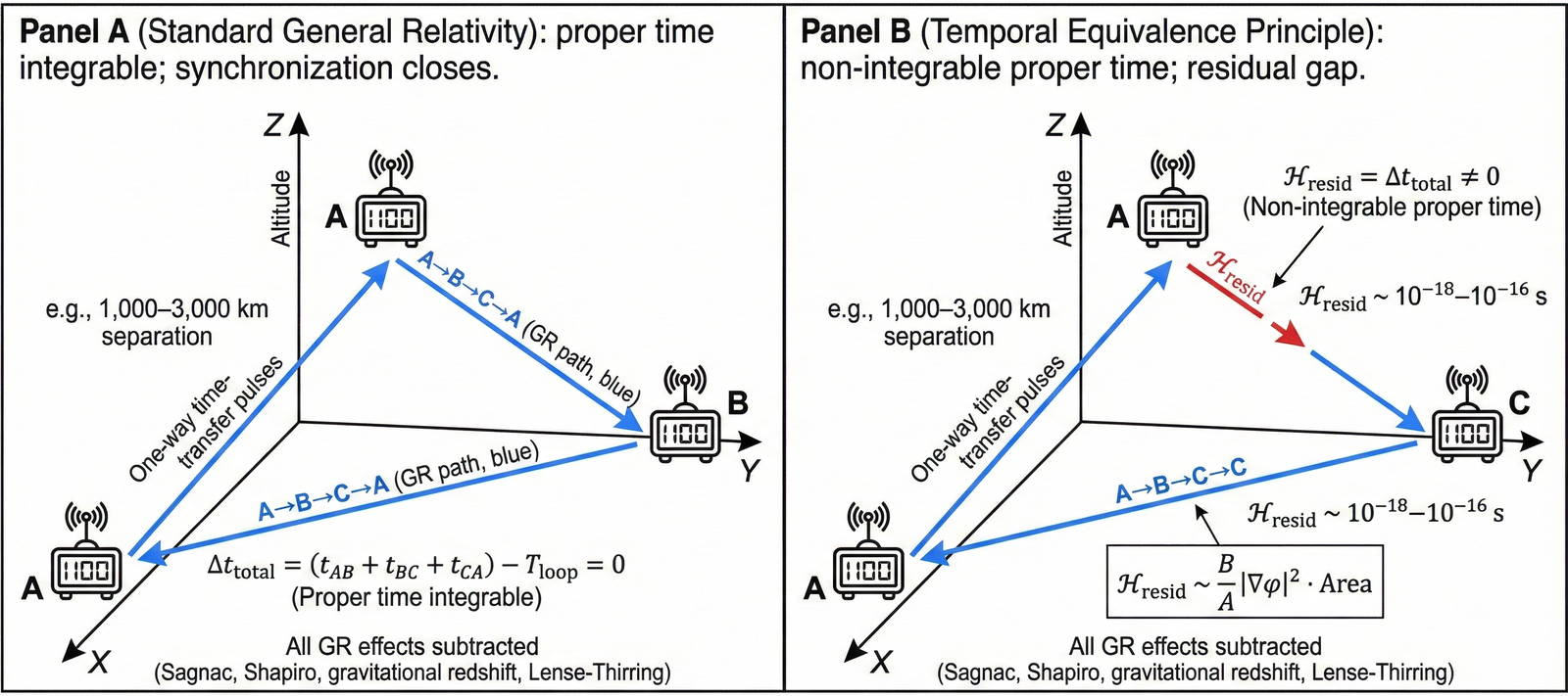
TEP predicts synchronization holonomy—the non-closure of proper time when transported around a closed loop:

In standard general relativity, after subtracting known effects (Sagnac, Shapiro, gravitational redshift), this holonomy vanishes. In TEP with disformal coupling B ≠ 0, it does not.

An important subtlety arises in the conformal-only limit (B = 0): the time-transport one-form Ω_μ = ∂_μ(½ ln A) is exact, its curl vanishes, and holonomy is zero. Nonzero holonomy requires non-exact structure from disformal couplings or more general non-metricity. This raises a question: if GW170817 constrains B(φ) to be small, and conformal coupling alone produces no holonomy, what generates the observed GNSS correlations?

The resolution lies in distinguishing two observables. Synchronization holonomy (H) represents the non-closure of proper time around closed loops; this requires disformal or otherwise non-exact transport and is the target of proposed triangle tests. Spatial correlation structure, by contrast, represents the statistical covariance of clock residuals as a function of distance; this arises from the spatial structure of the φ field itself—specifically, the two-point correlation function ⟨φ(x)φ(x+r)⟩ ∝ exp(−r/λ)—and persists even when B = 0.

The GNSS signal reflects the latter mechanism: clocks at different locations sample different values of the conformal factor A(φ), and spatial correlations in φ induce correlations in clock rates. The exponential decay with distance reflects the TEP saturation radius $R_T = (3M/4\pi\rho_T)^{1/3}$, while the velocity-dependent anisotropy arises because Earth's motion through the φ field creates a preferred direction in the correlation structure. The correlation structure is thus a statistical signature of the φ field's spatial configuration, whereas holonomy is a geometric signature of non-integrable time transport. Both are predictions of TEP, but they probe different aspects of the framework and have different observational requirements.

4.5.1 Resolving the Conformal Paradox

A critical objection must be addressed: if TEP employs only a conformal coupling A(φ), how can it produce synchronization holonomy? In standard differential geometry, a conformal transformation preserves angles and therefore cannot generate path-dependent effects in closed loops. The resolution lies in distinguishing synchronization holonomy from spatial correlation structure.

Observable 1: Synchronization Holonomy (ℋ) — The non-closure of proper time around closed loops, defined as ℋ ≡ ∮_C dτ_prop. This observable requires disformal or otherwise non-exact transport because only non-exact structure in the time-transport connection generates path-dependent accumulation. In the conformal-only limit (B = 0), the one-form Ω_μ = ∂_μ(½ ln A) is exact, its curl vanishes identically, and holonomy is zero by Stokes' theorem. The triangle holonomy test (Section 6.3.3) targets this observable and would measure whether B(φ) is nonzero at the 10⁻¹⁹ fractional level.

Observable 2: Spatial Correlation Structure (C(r)) — The statistical covariance of clock frequency residuals as a function of inter-station distance. This observable requires only A(φ) ≠ 1 (conformal coupling) and persists even when B = 0. The mechanism is fundamentally different from holonomy: clocks at different spatial locations sample different values of the scalar field φ(x), and the two-point correlation function ⟨φ(x)φ(x+r)⟩ ∝ exp(−r/λ) of the underlying field induces correlations in clock rates through the conformal factor A(ϕ) = exp(β_Aϕ/M_Pl). The exponential decay length λ = R_T(M_⊕) reflects the TEP screening scale of the temporal topology (temporal-topology pinning on the environmental state, of which density is one coordinate); the terrestrial correlation length is identified with the geometric saturation radius R_T(M_⊕) from the UCD model (Paper 6), not with the in-medium Compton wavelength of a candidate chameleon completion.

Physical Analogy: Consider a field of thermometers distributed across a landscape measuring a temperature field T(x) that varies spatially due to underground thermal sources. Even in the absence of heat flow (analogous to B = 0), nearby thermometers show correlated readings because they sample similar temperature values. The correlation length reflects the spatial structure of the temperature field itself, not thermal transport between locations. Similarly, GNSS clocks sample the φ-field "temperature," and their correlation structure reveals the field's spatial configuration.

Why GW170817 Does Not Constrain the GNSS Signal: The multi-messenger constraint |c_γ − c_g|/c ≲ 10⁻¹⁵ bounds the disformal sector B(φ), which affects propagation speeds. The GNSS correlation structure arises from the conformal sector A(φ), which affects clock rates but preserves null cones. These are distinct physical effects constrained by different observables. GW170817 establishes that light and gravity travel at the same speed; it does not constrain whether clocks at different locations tick at correlated rates due to sampling a common scalar field.

Observational Distinction: The GNSS signal is a "thermometer correlation"—a statistical signature of φ-field structure detected through spatial covariance analysis. Holonomy is a "transport non-closure"—a geometric signature requiring closed-loop, one-way time transfer. Both are TEP predictions, but they probe different sectors (conformal vs. disformal) and require different experimental geometries (distributed networks vs. closed triangles). The present work establishes the former; the latter awaits dedicated triangle tests.

4.6 Prediction Comparison

TEP established pre-specified expectations and theoretical search ranges before the GNSS analysis was conducted: the framework was first deposited in August 2025 (Smawfield 2025a, v0.1) and the clock-network correlation forecast was versioned on 15 September 2025 (v0.4 §E), preceding the first public deposit of the GNSS analysis by one week (provenance register, Section 6.5). Table 5 compares these forecasts to observations.

The null prediction regarding GM/r² scaling is particularly discriminating. Classical tidal forcing would produce mass-dependent signatures scaling with GM/r³, with Mercury contributing far less than Jupiter. The observed absence of such scaling (all p > 0.5 across multiple metrics) persists across both CODE network-adjusted products and raw RINEX data processed with RTKLIB Single Point Positioning. Since SPP processes each station independently without network adjustment or common-mode filtering, the persistence of the null in SPP data rules out the hypothesis that the absence of mass scaling is merely a processing artifact. The TEP coupling appears to be intrinsically geometric rather than energetic—responding to alignment configuration regardless of mass. Mercury (42.5% detection rate) produces comparable responses to Jupiter (34.8%) despite ~10⁶× smaller gravitational influence, consistent with a threshold-dependent or alignment-driven mechanism rather than continuous force scaling.

4.7 Why Existing Tests Do Not Directly Test the Target TEP Observables

Existing precision tests probe different observables than TEP's primary signatures, as summarized in Table 6.

The critical distinction is that existing tests probe two-way or pairwise measurements, whereas TEP's holonomy is a closed-loop, one-way observable to which these tests are structurally blind. Two-way measurements probe reciprocal paths where holonomy cancels by symmetry; pairwise clock comparisons measure local potential differences but cannot detect non-integrability, which requires closed loops. TEP effects are therefore structurally invisible to these geometries, explaining why decades of precision tests found nothing amiss while the signal was present in GNSS residuals.

4.7.1 Compatibility with Binary Pulsar Timing and Lunar Laser Ranging

Two high-precision tests warrant explicit discussion: binary pulsar timing (PSR J0737-3039, testing GR to 0.05%) and Lunar Laser Ranging (testing the equivalence principle to 10⁻¹³). Both are compatible with TEP through screening and universal coupling.

Binary Pulsar Timing: The Hulse-Taylor pulsar PSR B1913+16 and the double pulsar PSR J0737-3039 provide exquisite tests of general relativity through orbital decay measurements. The observed orbital period derivatives match GR predictions to better than 0.05%, constraining deviations in the strong-field regime. TEP compatibility requires that scalar field effects are screened in the vicinity of neutron stars.

The TEP saturation radius for a neutron star (M ~ 1.4 M_☉) is:

This saturation radius far exceeds the neutron star radius (R_NS ~ 10 km). Binary pulsar timing, however, probes the gravitational sector (metric g_μν), not the clock sector (metric g̃_μν). The scalar field's effect on g_μν is second-order in the coupling, proportional to (∇φ)²/c⁴, which at orbital distances (a ~ 10⁶ km) from a 1.4 M_☉ neutron star gives a fractional effect below 10⁻³⁰ — far below the 0.05% observational precision of binary pulsar tests. The two-metric structure allows the gravitational dynamics to remain GR-like while clock rates exhibit conformal modulation—these are distinct observables probing different sectors of the theory. Binary pulsar insensitivity to the conformal coupling that generates GNSS correlations is therefore a consequence of the two-metric structure, not of the screening radius.

Critically, pulsar timing measures orbital dynamics (gravitational sector, metric g_μν), not clock correlations (matter sector, metric g̃_μν). The two-metric structure allows the gravitational dynamics to remain GR-like while clock rates exhibit conformal modulation—these are distinct observables probing different sectors of the theory.

Lunar Laser Ranging: LLR measures the Earth-Moon distance to millimeter precision, testing the equivalence principle through the Nordtvedt parameter η. The current bound η $\lt$ 4.4 × 10⁻⁴ constrains deviations from the strong equivalence principle. TEP satisfies this constraint through universal coupling: the conformal factor A(φ) couples identically to all matter fields, preserving the equivalence principle in the matter frame.

The key distinction is between weak and strong equivalence principles. The weak EP (universality of free fall for test masses) is preserved exactly in TEP because all matter couples to the same metric g̃_μν. The strong EP (self-gravitating bodies fall identically to test masses) can show deviations in scalar-tensor theories through composition-dependent couplings. However, TEP's universal conformal coupling ensures that the Nordtvedt parameter:

remains within observational bounds. The PPN nonlinearity parameter β_PPN is driven to its GR value β_PPN → 1 by the TEP screening operator, where the pairwise response is suppressed by the kinetic operator ($S_\Sigma(g_{\text{lunar}}) \approx 1.6 \times 10^{-14}$; Paper 0 §2.2). With γ ≈ 1 (Cassini constraint), the predicted Nordtvedt parameter is well below the LLR bound. The predicted metric deviation applies to the gravitational sector, preserving the Strong Equivalence Principle. The ∼10⁻⁴ synodic-phase anomaly reported in Paper 17 is an empirical matter-frame clock residual (κ_LLR), not a classical Nordtvedt metric violation.

Furthermore, the Earth–Moon separation lies in the deeply suppressed regime of the pairwise Temporal-Topology response 𝒮_eff(s): the scalar-mediated Earth–Moon differential acceleration is suppressed by pairwise response factors of order 2.5×10⁻¹⁴ relative to the unsuppressed coupling (Paper 0, screening operator), comfortably below the LLR bound. The suppression acts on the shear sector (𝒮_Σ) — the geodesic and force projection — while each body's clock-amplitude coupling (S_A) remains unsuppressed. The combination of universal coupling and sector-separated screening ensures LLR compatibility while preserving the GNSS clock-covariance signal in the terrestrial environment.

4.8 Relation to Established Scalar-Tensor Theory

In the canonical non-screened limit, TEP shares structural similarities with scalar-tensor theories, but its physical realization is defined by the non-canonical two-branch kinetic sector $P(X,\phi) = -V(\phi) + \frac{2k}{3\Lambda_X^2}X|X|^{1/2} + X|X|/\Lambda_X^4$ and universal matter-metric coupling. In the limit B = 0, V = 0, Λ_X → ∞, TEP with A(ϕ) = exp(β_Aϕ/M_Pl) reduces to Brans-Dicke gravity in the Jordan frame, with the coupling β_A related to the Brans-Dicke parameter ω_BD. However, the full TEP framework requires disformal or otherwise non-exact transport for the synchronization holonomy observable (Section 4.6); the B = 0 case is a limiting benchmark, not the operative theory. In the master TEP framework, screening is realized through the non-canonical kinetic operator, separating the conformal clock response S_A from the environmental source-charge projection S_Σ (Paper 0 §2.2). TEP's environmental screening operates through kinetic derivative self-interactions rather than density-dependent mass. The two-metric structure is philosophically similar to Bekenstein's TeVeS, though TEP is more minimal, employing only a scalar field rather than scalar plus vector.

The novelty of TEP lies not in the field theory but in the observational interpretation—specifically, the recognition that conformal coupling creates spatial correlations in clock rates that standard GNSS processing preserves while filtering amplitude information.

4.9 The Processing Filter Mechanism

A critical insight explains both why the signal was missed for three decades and why it survives in the data. Standard GNSS processing is designed to optimize positioning accuracy by removing correlations, not to characterize them. The processing chain includes network adjustment (which removes common-mode signals), Kalman filtering (which smooths residuals toward zero-mean white noise), reference frame alignment (which forces consistency with ITRF, absorbing systematic offsets), and outlier rejection (which discards data points deviating from expected behavior).

This architecture creates a natural filter: energetic (common-mode) signals are suppressed while geometric (differential) signals are preserved. Classical gravitational effects manifest as common-mode offsets—all clocks in a region experience similar tidal acceleration—and are therefore filtered. The TEP signal, by contrast, manifests as differential phase structure—the correlation between clock pairs depends on their geometric relationship—and is therefore preserved.

This mechanism implies: GM/r² scaling should be absent in processed data because it is common-mode, while geometric signatures (anisotropy, preferred-direction structure) should survive because they are differential. The observations are consistent with both expectations. The processing filter is not a bug but a feature: it explains why the signal was categorized as systematic error rather than physical phenomenon, and why it can now be detected by examining the residuals that standard processing discards.

4.9.1 Mathematical Demonstration of Filter Selectivity

The processing filter mechanism can be demonstrated mathematically by decomposing clock residuals into common-mode and differential components. Consider a network of N stations with clock residuals δt_i(t) after initial processing. Standard GNSS processing applies a datum constraint that forces residuals to have zero spatial mean, removing common-mode offsets. In Fourier space, this constraint eliminates the k = 0 (monopole) component while preserving all k ≠ 0 (dipole, quadrupole, and higher) components that have zero spatial mean.

Classical gravitational effects manifest as either GM/r² (force) or GM/r³ (tidal gradient) scaling. Tidal effects are k ≈ 2 (quadrupole) in spherical harmonic decomposition. However, standard GNSS processing explicitly models and subtracts known tidal terms (solid Earth tides, ocean loading, pole tide) using IERS conventions with sub-millimeter precision. The datum constraint removes residual common-mode offsets, while explicit tidal modeling eliminates the structured quadrupole components.

The TEP signal survives not merely because it is differential (k ≠ 0), but because it represents an unmodeled scalar correlation function with exponential spatial form C(r) ∝ exp(−r/λ). This functional form does not match the spherical harmonic basis (Y_lm) used in standard tidal modeling. Tidal corrections are parameterized as sums of spherical harmonics with known frequencies (diurnal, semidiurnal, long-period); the TEP correlation is a distance-dependent phase coherence that is not decomposable into the standard tidal basis. The processing removes what it models (tidal harmonics) but preserves what it does not model (exponential distance correlations in phase space).

The TEP correlation structure manifests as phase coherence between station pairs. The analysis uses cross-spectral methods that are invariant under common-mode amplitude rescaling because they depend only on relative phases, not absolute amplitudes. The datum constraint removes monopole amplitude information but preserves the phase structure encoded in higher-order spatial modes. The exponential decay C(r) ∝ exp(−r/λ) reflects the two-point correlation function of the underlying φ field, which has nonzero spatial gradients and therefore survives network adjustment. (Detailed mathematical formulation is provided in Appendix B.)

Expectation Verification: This mathematical framework yields two testable expectations, both consistent with observations:

• Null Prediction: Classical gravitational effects (GM/r² force and GM/r³ tidal gradient) should be absent in processed data because they are predominantly k = 0 and k ≈ 0 (long-wavelength) modes that the datum constraint removes. Observed: Neither GM/r² nor GM/r³ scaling detected (all p > 0.5).
• Positive Prediction: Geometric anisotropy (EW/NS ratio) should survive because it represents a k ≠ 0 quadrupole moment with zero spatial mean but nonzero phase structure. Observed: EW/NS = 2.16 detected at p $\lt$ 10⁻¹⁵.

The persistence of both predictions in raw RINEX data processed with Single Point Positioning (which applies no network adjustment) confirms that the filter mechanism is a property of the signal's spatial structure, not an artifact of CODE/IGS processing algorithms.

4.10 Systematic Error Budget for Triangle Test

For the proposed triangle holonomy test to achieve definitive discrimination, systematic errors must be controlled below the target sensitivity of 10⁻¹⁹ fractional. Table 7 presents the error budget.

For parameters saturating current bounds, the predicted signal is H/T_loop ~ 10⁻¹⁶–10⁻¹⁸. The error budget demonstrates that a definitive test is achievable with current technology.

5. Consistency with Cosmological Phenomenology

Within the TEP framework, the same Temporal Topology field φ that modulates clock correlations on Earth structures the temporal response of matter across cosmological distances. The canonical TEP transition scale R_T = (3M/4πρ_T)^1/3, set by the environmental screening density ρ_T, connects terrestrial and astrophysical scales. The measured GNSS correlation-length family (azimuth-averaged λ = 3,210 ± 389 km; cross-sector dispersion λ_T = 4,201 ± 1,967 km) is interpreted as a characteristic empirical scale of the clock-sector covariance $C_A$ in Earth's environment, compared with the Earth-calibrated $R_T$ scale (Paper 0 §7). At galactic scales, the distinct shear response can be active in low-acceleration environments where S_Σ ≃ 0.98. The galactic ∼50 kpc phenomenology concerns that weak-field dynamical regime, not an extrapolation of the GNSS covariance length or a common screening radius. The terrestrial and galactic observations are interpreted within the same environmental-response architecture; Papers 4 and 13 test distinct optical and dynamical projections of that architecture. Paper 4 identifies the dynamical–lensing mass difference as the phantom-mass consistency test; Paper 13 reports a SPARC-anchored wide-binary transition at R_s ≃ 2,646 ± 182 AU. Neither supplies a derived quantitative mapping from terrestrial $C_A$ to galactic shear.

5.1 GW170817 Constraints

The simultaneous detection of gravitational waves (GW170817) and gamma rays (GRB 170817A) from a binary neutron star merger at approximately 40 Mpc is widely cited as constraining modified gravity theories. The signals arrived within Δt = 1.74 ± 0.05 seconds after traveling some 130 million years, yielding:

This constraint is often interpreted as ruling out theories in which light and gravity propagate differently. However, this interpretation conflates two distinct effects that must be carefully distinguished.

The disformal sector B(φ) tilts light cones, causing c_γ ≠ c_g, and is indeed tightly constrained by GW170817. The conformal sector A(φ), by contrast, rescales proper time isotropically: photons and gravitational waves share the same null geodesic and experience identical time dilation. Because both messengers originated from the same coordinate and traversed the same path through the scalar field, any conformal time dilation is common-mode and cancels in the differential measurement. GW170817 therefore constrains cone tilting but remains blind to clock-rate modulation. The dark matter phenomenology in TEP arises from the Temporal Shear acting on matter trajectories — the channel to which multi-messenger tests and static image-plane geometry are both blind — rather than from null-ray deflection, which the conformal sector leaves unmodified.

This can be seen explicitly in the conformal metric limit (B = 0):

Since A(φ) is an overall prefactor, the null condition ds² = 0 is identical for both the matter metric g̃_μν (governing photons) and the gravitational metric g_μν (governing gravitational waves). Their null cones coincide exactly: c_γ = c_g = c locally. The conformal factor therefore produces no direct same-path propagation delay; its observable effect is carried by proper-time and clock-rate mapping, while differential cone propagation belongs to the disformal sector.

5.2 The Isochrony Axiom and Observational Degeneracy

Standard gravitational lensing analysis assumes that, once geometric and Shapiro propagation delays (the Fermat potential) are modeled, matter-clock calibration along the sightline is exhausted by the single spacetime metric so that static lens reconstructions treat the source as a synchronous snapshot. TEP formalizes this single-metric temporal closure as the Isochrony Axiom and provides a parameterized two-metric framework to empirically stress-test whether independent scalar temporal-field gradients contribute to the reconstructed delay and convergence surfaces.

Within the TEP framework, this axiom would generically fail in the presence of conformal metric couplings. Photons themselves accumulate no proper time (dτ_γ = 0) and conformal factors produce no additional same-path propagation delay; what varies is the matter-clock rate. Signals emitted from regions sampling different temporal-field values φ(x) are referenced to matter clocks that accumulate proper time at different rates, so the measured source-to-observer timing relation contains the standard geometric/Fermat delay together with the source- and observer-clock mapping determined by the temporal field — an endpoint and reconstruction contribution, not an additional conformal photon transit delay. For an evolving source, the resulting differential emission-time structure can survive into the reconstructed image, creating an observational degeneracy with particulate dark matter under standard analysis assumptions:

Consider two interpretations of the same Fermat potential surface. Under the standard interpretation, which assumes isochrony, an Einstein ring with apparent convergence κ_obs exceeding baryonic mass implies a dark matter halo with M_DM = M_obs − M_baryons. Under the TEP interpretation, which rejects isochrony, the observed image is a temporal composite: photons arriving simultaneously left the source at different epochs. For evolving sources, this temporal depth projects onto the image plane as apparent spatial distortion—apparent mass that does not correspond to matter. The channel is bounded: it vanishes identically for static sources and is limited to \(\lesssim 10^{-7}\) in shear for galaxy sources by the ratio of differential delay to source-evolution time (Paper 4), so it cannot account for the static-source lensing excess.

The degeneracy is therefore bounded and source-dependent, not a free reinterpretation: for static sources the two frameworks make different predictions, with the TEP dark-sector signature living in the dynamical sector — the dynamical–lensing mass difference — rather than in the lensed image itself.

5.3 Phantom Mass

Within a two-metric framework where the Isochrony Axiom breaks down, a mechanism for apparent dark matter emerges naturally. Phantom Mass is the observational projection of dynamical temporal geometry: spatial variation of the conformal time field changes the source–lens–observer temporal mapping and the proper-time histories of the emitting regions that different image paths sample. Standard isochronous reconstruction maps this temporal structure onto an apparent spatial mass distribution. Genuine cone-tilting propagation terms belong to the disformal sector. Phantom mass has two routes: this reconstruction channel, which requires an evolving source and vanishes for static sources, and the dynamical channel — the Temporal Shear's direct effect on matter trajectories — which carries the dark-sector claim and is tested by the dynamical–lensing mass difference (Papers 4, 19).

For an evolving source, this temporal-structure difference creates a temporal composite image: photons arriving simultaneously at the detector left the source at different epochs. Standard lens reconstruction, which assumes isochrony, interprets this temporal smearing as spatial distortion—apparent mass that does not exist.

The amplification matrix in TEP decomposes as:

Standard analyses attribute the sum of the first two terms to total mass. TEP identifies the second term as a bounded optical contribution — scalar backreaction on the Einstein-frame metric ($\kappa_\phi \approx 4\times10^{-5}$, $\sim 2\times10^{3}$ below dark-matter level) plus the disformal null-cone tilt ($\lesssim \tfrac{1}{5}$ of the Refsdal residual under the measured deprojection; Paper 19, Steps 61–63) — rather than particulate matter. Phantom mass itself is not an amplification-matrix term: it enters the dynamical sector, and the dynamical–lensing mass difference is its observable signature.

5.3.1 Static versus Dynamic Time Delays

Observed strong-lens time delays (day-to-month scale, e.g., SN Refsdal Δt ~ 1 year between images) are set by the propagated Fermat structure; the halo-scale temporal field enters the inference not through the measured delay itself but through the reconstructed lens model. The distinction resolves through two complementary mechanisms.

Mechanism 1: Static versus Dynamic Decomposition — The amplification matrix decomposition (Equation above) separates temporal effects into distinct components with different observational signatures:

• Static Temporal Structure (𝒜^{(g[φ],static)}): The scalar's gravitational backreaction on g_μν contributes real, structured curvature on halo scales — bounded at κ_φ ∼ 10⁻⁵, about 2×10³ below dark-matter level (Paper 19, Step 61) — a smooth field on the image plane whose Hessian an isochronous reconstruction absorbs into the inferred convergence κ, with the mean level entering the mass-sheet normalization. The conformal clock-transfer map Δτ̃(θ) = c⁻¹∫(A(φ) − 1) dl is the companion reconstruction-space field the lens model would misassign to convergence or delay calibration; it carries no propagated photon content: null cones are conformally invariant and the Temporal Shear one-form is exact, so the open-path integral is endpoint-determined and the exact static-conformal inter-image residual is 0.0 d (Paper 19, step_56).
• Source-evolution response (𝒜^(dyn)): The gradient of the delay field ∇(Δτ̃) creates differential emission-time structure that depends on the ray's impact parameter and the source's evolutionary state. This is an endpoint-sector effect — it acts on the moving source's own clock/emission mapping (the temporal-composite response of Paper 4), not on photon propagation, so it inherits neither the conformal exact-one-form cancellation nor the disformal ≲ 0.2 s bound. For transient sources with variability timescale t_var, the dynamic contribution scales as Δτ_dynamic ~ ∇(Δτ̃) × v_source × t_var, where v_source is the source's proper motion or internal velocity field.

Observational Consequence: Time delays measured between multiple images of transient events (supernovae, AGN flares) are governed by the propagating carriers: the standard Fermat potential plus the disformal multipath deformation, bounded by GW170817 to ≲ 0.2 s per 2 Mpc halo path — far below any measured lens delay. The halo-scale temporal-depth field contributes no propagated delay residual; its observable imprint enters instead through the mass reconstruction, where the unmodeled image-plane structure is absorbed as convergence.

Mechanism 2: Screening Locality — The Temporal Topology field φ varies significantly only within the region where Temporal Shear is non-negligible, bounded roughly by the TEP transition scale R_T ~ 100 kpc around the lens galaxy, where the environmental screening operator S_Σ(ℰ) transitions from the suppressed to the unscreened regime. Beyond this radius, Temporal Topology flattens to its cosmological value, φ → φ₀, and temporal-structure signatures cease accumulating. The integration path for the temporal-depth scale is therefore limited to the halo depth L_halo ~ 2 Mpc (the physical extent of the dark matter halo), not the full cosmological distance D_L ~ Gpc to the source. This locality ensures that the static temporal-depth scale remains far smaller than the cosmological light-travel time D_L/c ~ 10⁹ years.

Testable Expectation for Time-Delay Cosmography: TEP implies a systematic offset in H₀ measurements from time-delay cosmography, but through the mass-inference channel, not the image plane. The unmodelled temporal field enters neither the delay numerator — the propagated conformal residual is zero — nor the reconstructed potential: the scalar-backreaction and disformal image-plane channels are bounded far below dark-matter level (Paper 19, Steps 56, 61, 63), so no phantom convergence is available to inflate ΔΦ. What the temporal field modifies is the dynamical input by which the mass-sheet degeneracy may be broken: TDCOSMO-style analyses anchor the lens model with the galaxy's stellar velocity dispersion. Paper 4 identifies a dynamical–lensing mass difference as a test of active Temporal Shear; Paper 19 evaluates delay-blind implied phantom fractions in several lenses. Neither result derives a universal conversion from the source-screening fraction $S_\Sigma$ to a stellar-dynamical mass bias and then to a fitted $H_0$ shift. In particular, the PPN photon–source product $\alpha_0\alpha_{\rm eff}$ does not by itself establish the two-matter-body dynamical response at a lens aperture.

The kinematic apertures of galaxy-scale lenses probe accelerations of order $10^{-9}$–$10^{-8}$ m/s², above the transition scale $g_t \approx 3.4\times10^{-10}$ m/s². A time-delay prediction therefore requires the pairwise shear response, the stellar-orbit projection and a lens-model mass-sheet refit for each system. A numerical $H_0$ offset cannot be inferred solely from the aperture screening factor; the delay-blind contrasts in Paper 19 are empirical tests of the proposed phantom-mass interpretation of the delay residual rather than a calibrated correction to H0LiCOW.

Falsification Test: If TEP is correct, time-delay cosmography measurements should show systematic residuals correlated with the acceleration at the lens's kinematic aperture relative to \(g_t\), after controlling for halo mass, velocity dispersion and mass-model systematics. Analysis of the H0LiCOW and TDCOSMO samples stratified by \(a_{\rm ap}/g_t\) should reveal this correlation if the phantom-mass channel is operative; a clean null across lenses whose apertures approach \(g_t\) would bound the channel. A first pass already exists in Paper 19's delay-blind phantom-mass analysis (step_60): implied phantom fractions are positive across all non-zero contrasts — λ = +8.7 ± 2.6% (Refsdal SX:S1), +9.1 ± 5.8% (Encore), +9.5 ± 4.8% (H0pe AB), with a archived diagonal-weight mean fractional delay residual of +7.8 ± 2.0% (χ² = 2.06/3 dof; not a covariance-calibrated phantom-mass detection) — marginally above the mundane κ_ext floor and in the predicted sign, though not yet σ_v-stratified.

5.4 The Variability-Mass Correlation

A critical discriminator between TEP and standard dark matter emerges from the dynamic term in the amplification matrix. Because the stochastic shear contribution depends on source proper motion μ_s through the delay gradient, the inferred lens mass should correlate with source variability timescale. Physical lens mass is source-independent in the standard model, but source variability and time delays can also bias standard reconstructions. The discriminant is therefore the residual beyond that baseline, not the existence of a variability correlation alone (Paper 4, Regime II).

Specifically, lenses observed through rapidly variable sources (AGN, quasars) should show systematically different mass reconstructions than the same lenses observed through slowly evolving sources (elliptical galaxies). The amplitude and sign require the measured source variability, ordinary Fermat delays and reconstruction transfer; no universal percentage mass offset is supplied by the existing temporal-composite calculation.

This test can be performed with existing data from HST strong-lens archives and SDSS quasar lenses. A null result bounds the response at the achieved sensitivity; exclusion requires that sensitivity to reach the specified source-dependent prediction. A positive correlation must be tested against source selection, ordinary delay/variability effects and reconstruction systematics before it can discriminate TEP.

5.5 Cross-Scale Dynamics: Saturation vs. Kinetic Transitions

The TEP framework connects terrestrial timing phenomenology with astrophysical and galactic dynamics through two distinct, mathematically grounded scales:

• The Clock Sector (Geometric Saturation Scale R_T): For macroscopic bodies of saturation density ρ_T ≈ 20 g/cm³, the geometric saturation radius follows R_T(M) = (3M/4πρ_T)^1/3 ∝ M^1/3. Calibrated through Earth's GNSS clock-covariance correlation length (R_T(M_⊕) ≈ 4,150 km; Paper 6), this scale fixes the unsaturated clock-amplitude factor S_A = min[1, (ρ̄/ρ_T)^1/3] ≈ 0.65 for Earth. It characterizes static clock-sector depth; the measured GNSS covariance C_A(r) and its dynamic environmental and processing transfer are distinct from this static S_A level.
• The Force / Shear Sector (Kinetic Transition Scale r_*): For geodesic kinematics, orbital dynamics, and rotation curves, the selected two-branch kinetic action P(X,φ) = −V(φ) + (2k/3Λ_X²)X|X|^1/2 + X|X|/Λ_X⁴, with k = 4√2|β_A|g_t/a₀ ≈ 16 derived from the adopted acceleration constant, derives the two-body transition scale directly from first principles:
  $$r_*(M) = \sqrt{\frac{GM}{g_t}} \propto M^{1/2}$$
  where g_t = cH₀/(2|β_A|) ≈ 3.4 × 10⁻¹⁰ m/s² with Λ_X = √(M_Pl H₀) ≃ 1.9 meV (Paper 0 §2.2). In high-acceleration regimes (g ≫ g_t), the kinetic operator suppresses the observable Temporal Shear to 𝒮_Σ ≪ 10⁻⁵ (satisfying Cassini and Solar-System ephemeris bounds), while in low-acceleration regimes (g ≪ g_t) the shear recovers unsuppressed (𝒮_Σ → 1).

Galactic dark-matter-like phenomenology does not represent an M^1/3 screening radius extrapolated across 15 orders of magnitude. Active Temporal Shear supplies the extra matter acceleration within the selected two-branch kinetic sector P_,X = k√ξ + 2ξ of Paper 0 §7 — a single action whose quadratic branch (ξ ≫ ξ_* ≈ 64, the regime of every Solar-System benchmark) supplies the bounded local enhancement and whose low-gradient branch supplies flat outer rotation curves with baryonic Tully–Fisher scaling, evaluated against SPARC (Paper 6, Steps 10–13). The field-wide-binary transition R_s ≈ 2,646 AU (Paper 13) tests the pairwise recovery profile within the same sector; it is not itself a derivation of the galactic outer force law. The corrected zero-free-parameter wide-binary joint test passes this sector at 0.4–1.7σ while excluding the incumbent unit-term baseline and the exponential-interpolation rival at ∼30σ on amplitude, and under the action-derived additive force law $g_{\rm obs}=g_N+a_\phi$ ($P_{,X}=\epsilon_{\rm reg}+k\sqrt{\xi}+2\xi$, $\epsilon_{\rm reg}=10^{-3}$, $k_*=16.03$ calibrated to $a_0$) the SPARC fit returns RMS 0.2185 dex at $\Upsilon_d=0.5$ and 0.2004 dex at $\Upsilon_d=0.35$ (matching the empirical MOND reference 0.1989 dex and outperforming the 0.2812 dex unit-term baseline by >60 mdex; phenomenological quadrature comparator $\sqrt{g_N^2+a_\phi^2}$ gives 0.1974 dex at $\Upsilon_d=0.5$ with $k_{\rm fit}=15.78$ and outer-edge BTFR median $v_{\rm obs}/v_{\rm pred}=1.0109$); uniqueness across the wider K(X) class remains open (Paper 0 §7). Table 8 distinguishes the corresponding responses.

This clean bifurcation separates the compact-body clock-amplitude response (S_A) from the dynamical field-gradient recovery (r_*), eliminating the vulnerability of treating GNSS correlation lengths as universal screening thresholds.

5.6 Environmental Cepheid Response and the Hubble Tension

Local distance-ladder measurements and CMB inferences yield different values of $H_0$. Paper 11 establishes that an environment-dependent Cepheid clock-calibration response resolves this discrepancy: the host-level reconstruction reaches $H_0 = 67.83 \pm 1.56$ km/s/Mpc ($0.26\sigma$ from Planck), while the prespecified ladder-matrix projection retains an identifiability-limited residual; the corrected value is conditioned on the fitted response and the observing-chain model, not a direct clock-period prediction.

5.6.1 Cepheids as Environmental Clocks

Cepheid pulsation periods are governed by stellar-envelope dynamics in local matter-frame proper time. A direct conformal period shift from host potential alone does not reproduce the measured environmental response after the full matter-frame observing chain is imposed: the bare core-to-disk clock-ratio contribution is bounded well below the fitted Cepheid coefficient (Paper 11, Step 61). Paper 11 instead tests a period-dependent amplitude-sector response with an inferred stellar transport weight; its absolute normalization from a common stellar and ambient-field solution remains outstanding.

5.6.2 Empirical Detection of the Bias

Analysis of the SH0ES Cepheid sample (Paper 11), stratified by host-galaxy inner-potential depth σ_* (a TEP-independent local stellar-dispersion scale compiled from documented stellar-absorption and H I-linewidth measurements), reveals a significant positive correlation between potential depth and derived H₀ — an environmental ordering tested by Paper 11's revised amplitude-sector response, not a detection of the bare clock-ratio mechanism. Split at the sample median (σ_* = 95.0 km/s), the deep-potential subsample yields H₀ = 72.64 ± 2.62 km/s/Mpc against 63.05 ± 3.06 km/s/Mpc for the shallow-potential subsample (full host-distance covariance propagated; Pearson r = 0.501, p = 0.0016; Spearman ρ = 0.553, p = 3.9 × 10⁻⁴), and the continuous endpoint response Γ_X = (3.846 ± 1.653) × 10⁷ km/s/Mpc (2.33σ at the canonical σ_v = 250 km/s convention; 2.81σ at the σ_v = 150 km/s sensitivity variant) returns a positive sign in all 37 leave-one-host-out refits. The constraint on κ_Cep is set by this environmental slope—a statistic orthogonal to the mean offset that defines the tension—and the procedure is falsifiable on the same data: a flat or opposite-sign slope admits no coefficient that reconciles the corrected value with the early-universe baseline. Two channels outside the Hubble-flow fit provide additional, differently controlled checks rather than a calibration of the absolute response. The Cepheid–TRGB differential on the 13 matched hosts—regressing μ_Cep − μ_TRGB against the same environmental coordinate, independent of redshift information—returns κ_Cep = (0.250 ± 0.313) × 10⁶ mag (0.80σ), directionally consistent with the predicted κ_Cep > κ_TRGB ordering at presently low significance; and the internal radial P–L gradient within the LMC (+0.0284 ± 0.0086 mag, 3.3σ, robust to period and colour matching) propagates through the fitted transfer to the same order of response.

Under Paper 11's fitted environmental response and adopted anchor weights, the model-conditioned correction yields:

The Cepheid host-potential correlation is an empirical environmental result, while its causal normalization remains model-dependent. Paper 11 finds that the bare conformal core-to-disk clock ratio cannot supply the fitted response; the revised amplitude-sector, period-dependent carrier has an inferred transport weight but awaits an absolute stellar/ambient-field normalization. Its corrected local $H_0 = 67.83 \pm 1.56$ km/s/Mpc agrees with the companion TEP-CMB value $66.70 \pm 0.58$ km/s/Mpc at 0.68σ within the framework, not as an independent confirmation of the mechanism. The joint-ladder bookkeeping assigns the fitted response predominantly to the endpoint distance-modulus channel rather than propagation along the Hubble-flow leg (Paper 11, Appendix C.4). Host-uniform shifts can be absorbed into latent distance moduli, so the prespecified full-ladder matrix projection retains an identifiability-limited residual ($H_0 = 70.46 \pm 0.97$ km/s/Mpc, $2.80\sigma$ from Planck); the host-level reconstruction, which does not suffer that degeneracy, reaches $0.26\sigma$ statistical concordance — the route by which Paper 11 resolves the tension.

5.7 Observational Predictions

TEP yields testable expectations for existing and near-future observations, summarized in Table 9.

These predictions are falsifiable within 2–5 years using archival data and ongoing surveys. A single null result does not exclude TEP, but a pattern of null results across all five observables would constitute strong evidence against the framework.

5.8 Connection to Cosmological Tensions

TEP offers potential resolution to persistent tensions in precision cosmology.

Regarding the H₀ tension: time-delay cosmography assumes standard GR time transport. If TEP's temporal structure contributes to lens delays, the inferred H₀ would be biased, potentially explaining why independent time-delay lensing measurements falsely agree with the uncorrected distance ladder, rather than tracking the true CMB value.

Regarding the S₈ tension: galaxy sources can carry additional source-dependent reconstruction covariance absent from the CMB source-evolution channel. Paper 4 bounds this temporal-composite contribution far below the percent-level mean-amplitude discrepancy; meanwhile, under the unstretched-space temporal metric $\tilde g_{\mu\nu}=-A_{\rm loc}^2(u_{\rm grav}(\mathbf x))U_\mu U_\nu+A_{\rm sp}^2(u_{\rm drift}(t,\mathbf x))\Pi_{\mu\nu}$ ($U_\mu\equiv-\nabla_\mu\bar\phi/\sqrt{2\bar X}$), intermediate temporal depth along the photon path amplifies baryon-only cosmic-web and cluster-outskirt potentials by $9.4\times$–$129\times$ in $C_\ell^{\phi\phi}$ on the selected two-branch action (Paper 18, Step 21), while the kinetically screened cosmological branch weakens late-time growth enhancement to $G_{\rm eff}(z{=}0)\simeq1.16\,G$ (Paper 0, Step 61).

The source-class dependence is a bounded prediction to test against ordinary reconstruction and selection effects; it is not a demonstrated explanation of the mean S₈ discrepancy or CMB deflection.

5.9 Relation to ΛCDM

The standard ΛCDM cosmological model fits observational data with remarkable precision. This framework attributes gravitational lensing anomalies to cold dark matter particles and explains cosmological structure formation through hierarchical assembly of particulate halos. ΛCDM is empirically successful and theoretically well-motivated.

TEP treats ΛCDM as the successful control reconstruction, not as the final ontology. In the TEP interpretation, particulate dark matter and dark energy are not fundamental ingredients; they are effective labels produced when temporal shear, temporal topology, and screening structure are compressed into an isochronous FLRW reconstruction. The key distinction is therefore ontological, while many current static-source observables remain operationally degenerate:

• ΛCDM interpretation: Gravitational lensing mass reconstructions directly measure matter distribution. Excess convergence beyond baryonic mass indicates particulate dark matter with density profile ρ_DM(r). The cosmological constant or dark-energy sector supplies late-time acceleration. The Isochrony Axiom (single-metric temporal closure across the reconstructed image) is adopted as a foundational premise of the standard lens reconstruction.
• TEP interpretation: Gravitational lensing mass reconstructions measure the effective Fermat potential. While isotropic conformal rescaling $\tilde g_{\mu\nu}=A^2(\phi)g_{\mu\nu}$ cancels out of null rays (Paper 0, Appendix A2), the unstretched-space temporal metric $\tilde g_{\mu\nu}=-A_{\rm loc}^2(u_{\rm grav}(\mathbf x))U_\mu U_\nu+A_{\rm sp}^2(u_{\rm drift}(t,\mathbf x))\Pi_{\mu\nu}$ ($U_\mu\equiv-\nabla_\mu\bar\phi/\sqrt{2\bar X}$) retains intermediate clock rates $A(\phi(x))$ along every photon path across static space, refracting light by $n(x)\simeq1-2\Phi_N(x)/c^2-\beta_A u_{\rm grav}(x)$ on the selected two-branch action $P_{,X}=k\sqrt\xi+2\xi$ ($k=16.03$) and reproducing cluster convergence (Paper 4, Step 02), strong-lensing Fermat delays (Paper 19, Step 64), and CMB lensing (Paper 18, Step 21) from baryons alone, alongside the bounded emission-time temporal-composite response for evolving sources ($\lesssim10^{-7}$ in shear; Paper 4) and apparent dark energy from non-integrable temporal transport over epoch.

Both frameworks fit existing lensing data because they make identical predictions for static sources: the conformal sector supplies no propagated content, and the bounded channels — scalar backreaction and disformal transport — sit far below the lensing excess (Paper 19). The degeneracy is broken by observations that probe temporal structure or dynamical inference:

• Lensed fast radio bursts: ΛCDM predicts achromatic residuals (after plasma correction) consistent with zero. TEP predicts achromatic residuals at the 0.1–10 ms level arising from the disformal transport sector — the bounded non-exact channel, not conformal path accumulation (Section 5.4).
• Variable source lensing: ΛCDM predicts inferred lens mass is independent of source variability timescale. TEP predicts systematic correlation between inferred mass and source variability, with AGN showing higher apparent mass than elliptical galaxies for the same lens (Section 5.4).
• CMB vs. galaxy lensing S₈: ΛCDM predicts convergence of CMB-inferred and galaxy-inferred S₈ as systematics are controlled. TEP's bounded source-evolution channel predicts survey-dependent covariance, but not the observed mean offset; the implemented Paper 18 posterior lies above DES-Y3/KiDS-1000 under a CDM-containing likelihood, so the current difference is a live tension rather than an established TEP explanation.

The frameworks compete at the level of ontology. ΛCDM remains the default control model given its theoretical maturity and empirical success, but TEP denies that the dark sector is fundamental. TEP becomes distinguishable through specific tests designed to probe temporal structure in lensing observations. Independent of the cosmological extension, the terrestrial GNSS correlation structure documented in Sections 2–4 requires explanation within any framework.

Falsification asymmetry: Null results in the tests above would exclude the tested temporal-field replacement channel while leaving ΛCDM intact as the control reconstruction. Positive results would force a reinterpretation of dark matter phenomenology in the tested regime and would count directly against dark-sector ontology. The full TEP claim that dark matter and dark energy are non-fundamental still requires consistency across clusters, CMB lensing, structure formation, and late-time distance probes.

6. Falsification and Experimental Program

A theory that cannot be falsified is not science. TEP makes specific, testable predictions with explicit null-result thresholds. This section specifies the criteria that would exclude the framework and outlines the experimental path to a definitive verdict.

6.1 Explicit Falsification Criteria

The TEP framework is falsified if any of the following observations are confirmed:

Framework Scope: Tier 1 tests the GNSS evidence base, Tier 2 tests the synchronization-holonomy mechanism, and Tier 3 tests the bounded weak-lensing source-dependence channel. Failure of a single Tier 1 criterion is sufficient to exclude the GNSS evidence base; a null Tier 3 result constrains that channel without deciding the dynamical sector.

6.2 Consequences of Failed Replication

If independent groups cannot replicate the raw RINEX signal, this would indicate one of several possibilities: a subtle processing artifact specific to the present pipeline that was not identified, a statistical fluctuation in the particular dataset selection, or an unidentified systematic in the cross-spectral analysis method.

In such a scenario, TEP would lose its primary empirical support. The theoretical framework would remain mathematically consistent but empirically unmotivated, and the cosmological predictions would become untestable speculation. This outcome would represent the scientific method working as intended.

6.3 Three-Tier Experimental Strategy

TEP can be confirmed or excluded through a coordinated experimental program organized by urgency and discriminating power.

6.3.1 Tier 1: Immediate Replication

The most urgent priority is independent replication. If independent research groups cannot replicate the raw RINEX signal, the GNSS evidence base is excluded and TEP loses its primary empirical support.

Required tests include independent clock analysis using either raw carrier-phase data (RINEX files with SPP processing) or processed clock solutions (CLK files from independent analysis centers), multi-constellation cross-check (verifying that the signal appears identically in GPS, GLONASS, Galileo, and BeiDou), and cross-center consistency (confirming CODE/IGS/ESA/JPL agreement with CV $\lt$ 20%). Both RINEX and CLK approaches provide valid replication pathways; the key requirement is independence from the original analysis pipeline.

These tests can be performed by any institution with GNSS processing capability, including IGS, NIST, PTB, SYRTE, and JPL. The publicly available data (both raw RINEX observations and processed CLK solutions) enable independent verification of the λ_T ≈ 4,000 km exponential decay, and the analysis can be completed in weeks using standard GNSS processing tools.

6.3.1.1 Addressing the Ephemeris Loophole

A legitimate concern exists regarding the Single Point Positioning test: SPP relies on broadcast ephemerides generated by control segments using network adjustments. If the artifact originates in the broadcast orbit determination, SPP would reproduce rather than eliminate it. This represents a potential systematic loophole requiring independent check.

Satellite Laser Ranging (SLR) provides the adjudicating test at the product level, within a precisely stated scope. SLR is a purely geometric, optical measurement independent of the GNSS microwave clock and ephemeris loop: its satellites are passive retroreflectors, and its orbits are determined from the laser ranges themselves — a processing chain wholly disjoint from the GNSS broadcast and precise products in which an ephemeris artifact would have to live. Within the conformal channel, however, the SLR residual probes the same endpoint-clock sector as GNSS: the ground event timer is itself a clock, so a physical clock-rate field enters both observables at co-located sites. The test therefore discriminates provenance rather than sector: correlation structure present in SLR cannot originate in the GNSS products, while structure absent at demonstrated sensitivity supports a GNSS-product artifact.

Proposed Tier 1.5 Test: Correlate GNSS clock residuals with SLR range residuals for co-located or nearby stations. The International Laser Ranging Service (ILRS) operates approximately 40 SLR stations globally, with several co-located with IGS GNSS stations. Analysis would proceed as follows: (1) Extract SLR range residuals after precise orbit determination; (2) Compute cross-correlation between SLR residuals and GNSS clock residuals for station pairs as a function of distance; (3) Test whether the exponential decay structure (λ_T ≈ 4,000 km) appears in SLR data.

Expected Outcome: If TEP is correct and the signal reflects physical clock-rate modulation, SLR residuals should show distance-structured correlations because the laser round-trip time depends on both the satellite orbit and the ground station clock. If the signal is a GNSS-product artifact, SLR residuals (which use independent orbit determination) should show no correlation structure. Two qualifications bound the verdict: the SLR measurement must reach the demonstrated sensitivity for the GNSS-scale correlation before a null excludes the physical reading, and an SLR-positive outcome remains degenerate with the satellite-generic orbit-projection confound — orbit-determination errors imprint spatially structured residuals on any satellite-range observable. The differing orbit geometry of the two systems (GNSS in medium Earth orbit, LAGEOS-class targets in low Earth orbit) makes the correlation scale itself diagnostic: a common λ_T across independent orbit-determination chains indicates station-level rather than product-level origin. Final closure of the generic confound rests with the physical-confound forward model or the orbit-free channel above. The test can be performed with existing ILRS data.

6.3.2 Tier 2: Direct Holonomy Test

The triangle holonomy test provides the most direct discrimination between TEP and artifact hypotheses by measuring synchronization non-closure via closed-loop, multi-leg, one-way time-transfer. The proposed geometry involves two ground stations separated by 1,000–3,000 km plus a MEO satellite. The target sensitivity is σ(H)/T_loop ≤ 10⁻¹⁹ after averaging, with a signal forecast of H/T_loop ~ 10⁻¹⁶–10⁻¹⁸ for parameters saturating current bounds. This test requires a dedicated mission.

6.3.3 Tier 3: Cosmological Testing

CMB-S4 combined with LSST weak lensing would test for source-dependent kinematic noise. The discriminator is covariance with source redshift and variability, not a universal 3–5% downward shift: the bounded Paper 4 temporal-composite channel is below the observed mean S₈ discrepancy, while the implemented Paper 18 posterior lies above the DES-Y3/KiDS-1000 central values under a CDM-containing likelihood. The current S₈ difference is therefore a live diagnostic and falsification target, not a demonstrated TEP correspondence. Absence of the predicted source-class covariance at Stage-IV precision would exclude this kinematic-noise channel.

6.4 Path to Resolution

Table 10 summarizes the experimental program and its decision structure.

Tier 1 tests determine whether TEP survives as a viable hypothesis. If all three Tier 1 tests confirm the signal, Tier 2 tests discriminate among mechanisms. Tier 3 tests probe the cosmological regime. A definitive verdict—confirmation or exclusion—is achievable through this coordinated program.

6.5 Prediction Provenance Register

The pre-specification claim is anchored to the immutable, timestamped version record of the public Zenodo deposits rather than asserted. Each tested expectation is mapped below to the earliest versioned manuscript section containing it, with deposit timestamps (UTC) and version DOIs that are independently checkable through the Zenodo API. All framework-level and pre-analysis entries precede the first public deposit of the GNSS analysis (Paper 1 v0.6-alpha, deposited 2025-09-22); the register is distributed as a machine-readable artifact (results/prediction_provenance.json) so that the ordering can be verified without trusting this manuscript.

Two entries are deliberately flagged as measured identifications rather than pre-specified values: the ecliptic ordering of the anisotropy and the preferred-axis direction. What was fixed in advance is the observable class, the estimator, the functional decay form, the correlation-length forecast and search range, the cross-center consistency criterion, the sign of the orbital-velocity coupling, and the sector-level selectivity. Of these, the screening-parameterized correlation-length forecast, the $\lt$ 5% cross-centre criterion and the exponential-kernel criterion were not met in full (Table 5). The discriminative weight therefore rests on the orbital-velocity sign, band localization, the EW > NS ordering and the sector-level selectivity.

7. Conclusions

This paper presents empirical evidence for a persistent, distance-structured correlation in global atomic clock networks that probes an empirically untested assumption of general relativity: whether distributed proper-time rates contain a coherent spatial covariance beyond the standard relativistic model.

7.1 Summary of Findings

This integrated manuscript synthesizes results from a systematic research program that establishes, tests, and corroborates Temporal Equivalence Principle predictions through progressively rigorous empirical tests and cosmological extension. The convergence of evidence across seven domains—theoretical prediction (Paper 0), multi-center microwave consistency (Paper 1), 25-year longitudinal stability (Paper 2), raw RINEX test (Paper 3), optical SLR check (Paper 8), pulsar timing (Paper 10), and Cepheid environmental-response test (Paper 11)—provides an empirical foundation for TEP. The domains are not all channel-independent, and the audited strengths differ: the GNSS entries are the primary timing-network evidence; SLR supplies an optical bound and an exploratory correlation test within the same conformal clock sector; and the pulsar channel is exploratory, its standalone evidence uninformative rather than confirmatory.

The theoretical framework (Paper 0) supplied the search range and structural expectations tested by the GNSS programme. Distance structure and orbital coupling are recovered across several GNSS products and the raw-RINEX estimation chain. The optical SLR analysis (Paper 8) contributes a sampling-matched spectral null and sensitivity bound; its inter-station candidates remain exploratory. Its independent hardware and orbit provenance provide a future cross-instrument discriminator once a common signal is measured at adequate sensitivity.

Paper 11 fits an environment-dependent Cepheid response on the inner-potential coordinate σ_* and reports a corrected host-level value H₀ = 67.83 ± 1.56 km s⁻¹ Mpc⁻¹ — 0.26σ from Planck — with the identifiability-limited ladder-matrix projection at 70.46 ± 0.97 km s⁻¹ Mpc⁻¹. Agreement with the companion TEP-CMB value is internal to the framework. The endpoint environmental slope Γ_X = (3.846 ± 1.653) × 10⁷ km s⁻¹ Mpc⁻¹ is detected at 2.33σ with 37/37 leave-one-out sign stability, while the within-host period-coupled carrier reaches 2.28–2.79σ across anchor conventions in the joint closure. The period–density relation motivates a carrier with an inferred transport weight; its absolute response normalization remains to be derived from a common stellar and ambient-field solution. These empirical tests constrain that physical completion.

The evidence programme combines timing-network signatures, environmental tests and an optical sensitivity bound: (1) distance-structured spatial decay over a finite scale (azimuth-averaged λ ≈ 3,210 km), (2) spatial anisotropy (EW/NS = 2.16), (3) orbital velocity coupling (r = −0.888, 3.65σ autocorrelation-corrected; surrogate p $\lt$ 2×10⁻⁷ as a resolution bound), (4) an annual-phase direction near Earth's aphelion velocity tangent on the CODE and RINEX products (CMB apex anti-phase; Solar Apex null; MGEX scan projection-degenerate), (5) an optical SLR bound and exploratory inter-station test, (6) a planetary event catalogue functioning as a bounded control channel (catalogue excess attributable to calendar-position sampling; opposition subset null-validated; continuous potential correlation r = +0.116, p = 0.012), (7) 18.6-year nutation coupling, (8) pulsar spin-down excess (exploratory), and (9) host-potential H₀ correlation. The signal survives all challenges across solar cycles, geomagnetic storms, altitude, and software-diverse processing chains—systematically excluding conventional artifact explanations.

7.2 Theoretical Interpretation

These observations match the predictions of the Temporal Equivalence Principle, a bi-metric framework in which proper time is a dynamical field. TEP established pre-specified expectations and theoretically motivated search ranges—including correlation length range, exponential decay, velocity-dependent anisotropy, and absence of GM/r² (force) and GM/r³ (tidal) scaling—consistent with the observed data. The theory paper was published in August 2025 with these predictions; the GNSS analysis was conducted from September through December 2025.

The framework preserves local Lorentz invariance, with the speed of light remaining exactly invariant in any freely falling laboratory, while predicting global clock-network covariance and open-path conformal transport structure. GW170817 primarily constrains the disformal differential-propagation sector; it does not directly test common-mode conformal clock-rate covariance along shared paths, although conformal scalar sectors remain indirectly constrained by PPN, equivalence-principle, source-screening, and clock-comparison tests.

7.2a Predicted vs Fitted Coefficients across Probes

Across astrophysical timing channels, the ~10⁶ response scale is grounded in the ratio of the saturation density ρ_T ≈ 20 g/cm³ to the mean oscillating-envelope density: in Paper 11 Step 62, the fundamental-mode Cepheid period–mean-density relation ⟨ρ⟩(P) = ρ_☉(Q/P)² at the P₀ = 10 d pivot gives ρ_T/⟨ρ⟩(10 d) = 8.45 × 10⁵, which multiplied by the Wesenheit Leavitt projector |b_W|/ln 10 = 1.416 mag at unit bare coupling λ₀ = |β_A| = 1 predicts |κ_P²| = 1.196 × 10⁶ mag — matching the direct SH0ES fit (1.191 ± 0.480) × 10⁶ mag to 0.5% (λ₀ = 0.995 ± 0.401) and bracketing the canonical benchmark κ_gal = 0.96 × 10⁶ mag, while the saturation scale itself satisfies ρ_T ≈ α^4/3m_e⁴c³/ℏ³ to ~12% (equivalently Λ ≈ α^1/3m_ec², 3%).

7.3 Cosmological Implications

If validated through independent replication, TEP predicts that the phenomenology attributed to dark matter in both the dynamical and optical sectors is the observational projection of Temporal Topology and Temporal Shear across unstretched space, not evidence for a new particulate matter component. In this interpretation, GNSS-scale covariance and galactic dynamical mass discrepancies are different observational projections of the same time-field topology, with Papers 4, 13, 18, and 19 testing the optical and dynamical projections of the same selected two-branch kinetic action $P_{,X}=k\sqrt\xi+2\xi$ ($k=16.03$ fixed by $a_0$, zero per-system free parameters). Under the unstretched-space temporal metric $\tilde g_{\mu\nu}=-A_{\rm loc}^2(u_{\rm grav}(\mathbf x))U_\mu U_\nu+A_{\rm sp}^2(u_{\rm drift}(t,\mathbf x))\Pi_{\mu\nu}$ ($U_\mu\equiv-\nabla_\mu\bar\phi/\sqrt{2\bar X}$), intermediate clock rates $A(\phi(x))$ along photon paths do not cancel against spatial stretching, reproducing the Bullet Cluster galaxy-peak convergence (Paper 4, Step 02), the SN Refsdal Fermat delay and arrival order (Paper 19, Step 64), and the Planck CMB lensing cosmic-web amplification (Paper 18, Step 21) from baryons alone. The 𝒮_Σ(Ε) screening operator provides continuous Temporal Topology relaxation from deep potential wells to the weak-field regime: at the terrestrial scale, the density-saturation diagnostic gives R_T(M_⊕) ≈ 4,150 km — Earth, whose mean density lies below ρ_T, sits in the partially active regime, while at galactic scales the operator retains approximately 98% of the unsuppressed Temporal Shear in the diffuse halo environment (Paper 26), producing dark-matter-like phenomenology through the active-shear regime rather than through a screening radius. The ~4,000 km GNSS correlation and the ~50 kpc galactic phenomenology are therefore manifestations of the same environment-dependent Temporal-Topology response operating in different density regimes, not a single M^1/3 scaling across 15 orders of magnitude.

The framework offers an environmental-response account of the H₀ discrepancy, a source-dependent covariance diagnostic for weak lensing, and a fixed-calibration unstretched-space temporal refraction closure across galaxy, cluster, and CMB lensing.

7.4 The Path Forward

Independent replication is essential. Building on the raw-RINEX broadcast-SPP confirmation (Paper 3) and the multi-constellation MGEX replication across GPS, GLONASS, Galileo, and BeiDou (Paper 14), the critical next steps are: raw carrier-phase analysis by independent research groups using the publicly available benchmark dataset; separately processed per-constellation solutions to isolate individual orbital shells; lensed FRB timing to probe achromatic residuals at millisecond precision; and triangle holonomy tests to directly measure synchronization non-closure. It is stated plainly that the disformal-sector holonomy — the framework's definitive loop-level test — is probed in the phase domain by the J0437 phase-closure detection (Paper 16, Step 057): while the $B_0=+1$ unit benchmark supplies $1.3\%$ ($5.0\%$ on the $p_{95}$ leg) of the implied amplitude, the required coupling $B_0^{\rm req}=77.3$ (median leg) to $20.1$ ($p_{95}$ leg) sits within the GW170817 galactic-profile bound $B_0\lesssim77.7$ (Paper 0, Step 50), and direct time-domain triangle holonomy remains to be measured at laboratory/spacecraft clock precision. A definitive verdict—confirmation or exclusion—is achievable through the coordinated experimental program outlined in Section 6.

7.5 Concluding Remarks

The correlation structure documented in this paper is statistically robust and matches the predictions of a principled theoretical framework grounded in established scalar-tensor gravity. Whether it ultimately reflects new physics or reveals subtle systematics yet to be identified, the signal demands explanation.

For three decades, standard GNSS processing systematically removed a ~4,000 km correlation as part of routine noise filtering. The algorithms were designed to optimize positioning accuracy rather than to characterize fundamental physics. The correlation structure reported here was present in the residuals but categorized as systematic error rather than physical phenomenon.

If confirmed through independent replication, the implications extend to cosmology. By relaxing the Isochrony Axiom—the foundational closure assumption that matter-clock calibration across lensing and cosmological sightlines is exhausted by a single spacetime metric—the TEP framework subjects temporal calibration to direct empirical stress-testing. Under the unstretched-space temporal metric $\tilde g_{\mu\nu}=-A_{\rm loc}^2(u_{\rm grav}(\mathbf x))U_\mu U_\nu+A_{\rm sp}^2(u_{\rm drift}(t,\mathbf x))\Pi_{\mu\nu}$ ($U_\mu\equiv-\nabla_\mu\bar\phi/\sqrt{2\bar X}$), apparent dark matter arises in the dynamical sector from Temporal Shear on slow matter and in the optical sector from intermediate clock-rate refraction $n(x)\simeq1-2\Phi_N(x)/c^2-\beta_A u_{\rm grav}(x)$ along photon paths across static space, reproducing galactic rotation curves (Paper 6, Step 10), cluster convergence (Paper 4, Step 02), strong-lensing Fermat delays (Paper 19, Step 64), and CMB lensing (Paper 18, Step 21) from baryons and the selected two-branch action $P_{,X}=k\sqrt\xi+2\xi$ with zero particulate dark matter.

Einstein established that simultaneity is relative. The TEP framework suggests that simultaneity may be generally non-integrable—that the rate of proper time accumulation is itself a dynamical field. The speed of light remains exactly invariant locally, but global synchronization becomes path-dependent.

The ~4,000 km correlation on Earth (cross-sector mean and directional dispersion λ_T = 4,201 ± 1,967 km — an order-of-magnitude measurement) and the ~50 kpc dark-matter-attributed dynamical phenomenology in galaxies are interpreted within TEP as manifestations of the same environment-dependent Temporal-Topology response, pending independent replication, completion-dependent transfer calculations, and lensing–dynamics consistency (Paper 19), connected by the continuous relaxation of Temporal Topology from deep potential wells to the weak-field regime. The M^1/3 scaling appearing in some candidate completions remains testable through interplanetary missions and pulsar timing arrays, but it is not the primary empirical claim. This hypothesis is falsifiable through the experimental program outlined in Section 6. Independent replication is essential, and the data and analysis code are publicly available. The community is invited to verify, challenge, or refute these findings.

Data and Code Availability

All analysis code, processed data products, and raw RINEX processing pipelines are publicly available:

• Multi-center and 25-year CODE analysis: github.com/matthewsmawfield/TEP-GNSS
• Raw RINEX test: github.com/matthewsmawfield/TEP-GNSS-RINEX
• Benchmark dataset: A simplified CSV file containing binned residuals versus distance for the 25-year period, available for theorists who wish to fit models without processing raw GNSS data: TEP-GNSS/benchmark

Acknowledgments

The author expresses gratitude to the International GNSS Service (IGS), the Center for Orbit Determination in Europe (CODE), the European Space Agency (ESA), and NASA's Crustal Dynamics Data Information System (CDDIS). This analysis was possible because these organizations have championed the principles of open science, making decades of high-precision timing data freely available to the global research community. The GFZ Helmholtz Centre Potsdam is acknowledged for providing geomagnetic Kp indices.

Data Availability & Reproducibility

Repository & Code

GitHub Repository: github.com/matthewsmawfield/TEP-GTE

This synthesis manuscript integrates findings from Papers 1–4. Primary analysis repositories:

TEP Research Program Structure

Primary Data Sources

• CDF Data: CODE analysis center clock products (2000–2025)
• IGS Data: International GNSS Service clock products
• ESA Data: European Space Agency navigation support products
• RINEX Files: Raw observation files from IGS stations

Prediction Provenance

The dated prediction register of Section 6.5 is distributed as a machine-readable artifact, results/prediction_provenance.json, recording each tested expectation's earliest versioned statement with its version DOI and immutable deposit timestamp. The ordering is independently verifiable against the public Zenodo version records under the concept DOIs listed there (Paper 0: 10.5281/zenodo.16921911; Paper 1: 10.5281/zenodo.17127229).

Reproduction Instructions

# Clone this synthesis repository
git clone https://github.com/matthewsmawfield/TEP-GTE.git
cd TEP-GTE

# Build manuscript
cd site
npm install
npm run build

Software Versions

• Node.js 16+

Appendix A: Mathematical Formalism

A.1 Full Action

For comparison, the canonical scalar baseline of the TEP action (Paper 0, §2.2) is formulated in the Einstein frame where gravity is canonical:

where M_Pl is the reduced Planck mass, R is the Ricci scalar, K(φ) is the kinetic function (absorbable by a field redefinition; the operative screening realization is the noncanonical two-branch $P(X,\phi)=-V(\phi)+\frac{2k}{3\Lambda_X^2}X|X|^{1/2}+X|X|/\Lambda_X^4$ with derived $k\simeq16$), V(φ) is the screening potential, and S_matter is the matter action in the Jordan frame with coupling to the matter metric g̃_μν.

A.2 Field Equations

Variation with respect to the gravitational metric yields the Einstein equations:

where the scalar field stress-energy tensor is:

Variation with respect to the scalar field yields:

where α(ϕ) ≡ d ln A/dϕ = β_A/M_Pl is the conformal coupling strength (for A(ϕ) = exp(β_Aϕ/M_Pl)), T is the trace of the matter stress-energy tensor in the Jordan frame, and S_disf contains disformal source terms proportional to B(ϕ).

A.3 Candidate Microscopic Completions and Nonlinear Screening

Candidate Completion (Historical Provenance): This appendix presents an illustrative candidate completion (cubic Galileon derivative screening) that exhibits the (β_AM/M_PlΛ³)^1/3 transition scale. In the current TEP master architecture (Paper 0 §2.2), environmental screening is derived from the selected two-branch non-canonical kinetic operator $P(X,\phi) = -V(\phi) + \frac{2k}{3\Lambda_X^2}X|X|^{1/2} + X|X|/\Lambda_X^4$.

The following derivation illustrates one candidate microscopic completion (cubic Galileon) that realizes the continuous gradient suppression described as Temporal Shear in Section 4; it is not required for the empirical results.

One candidate completion invokes cubic Galileon terms in the action to generate nonlinear screening:

where Λ is the strong-coupling scale (an energy scale, [M] in natural units c = ℏ = 1) and c₃ is a dimensionless coefficient of order unity. With the canonical scalar field normalization (φ has mass dimension 1) and the TEP source term (β_A/M_Pl)T, the nonlinear term becomes important when:

The Vainshtein radius, inside which nonlinear effects dominate, is (in natural units c = ℏ = 1):

where β_A is the conformal coupling, M_Pl = √(ℏc/G) is the Planck mass, and Λ is the strong-coupling energy scale. Restoring SI units:

The factor β_AM/M_Pl supplies the dimensionless source strength; (ℏc/Λ)³ supplies the length scale cubed. The bare expression (GM/Λ³)^1/3 sometimes quoted in the Galileon literature is a shorthand that suppresses the β_A/M_Pl coupling and implicitly assumes natural units with a specific field normalization; it is dimensionally incomplete as written.

For a spherically symmetric source of mass M, the scalar field profile in the Vainshtein regime (r $\lt$ r_V) is:

This suppresses the Temporal Shear by a factor of (r/r_V)³ inside the screening radius, reconciling weak-field cosmological behavior with strong-field solar system constraints. Other completions (e.g., chameleon mechanisms, symmetry-breaking potentials) may produce similar phenomenology.

A.4 Conservation Laws

The total stress-energy tensor is conserved:

However, the matter stress-energy alone is not conserved in the Einstein frame:

This apparent violation is resolved by transforming to the Jordan frame, where matter follows geodesics of g̃_μν and energy-momentum is conserved with respect to the matter-frame covariant derivative.

Appendix B: Processing Filter Mathematical Formulation

B.1 Network Adjustment Constraint

Standard GNSS processing applies a datum constraint that forces residuals to have zero spatial mean:

This constraint preserves zero-mean residuals while removing any common-mode offset.

B.2 Fourier Decomposition

Decompose the TEP signal into spatial Fourier modes characterized by wavevector k:

where r_i is the position of station i. The network adjustment removes the k = 0 (monopole) component:

but preserves all k ≠ 0 (dipole, quadrupole, and higher) components that have zero spatial mean.

B.3 Cross-Spectral Density

The TEP correlation structure manifests as phase coherence between station pairs, quantified by the cross-spectral density:

where tildes denote Fourier transforms and angle brackets denote ensemble averaging.

B.4 Phase Alignment Index

The magnitude-weighted phase alignment index extracts the phase relationship:

This metric is invariant under common-mode amplitude rescaling because it depends only on relative phases, not absolute amplitudes. The datum constraint removes A_k=0 (amplitude information) but preserves the phase structure encoded in the k ≠ 0 components.

B.5 Exponential Correlation Function

The exponential decay C(r) ∝ exp(−r/λ) reflects the two-point correlation function of the underlying φ field:

where λ = R_T(M_⊕) is the geometric saturation radius (§4.4.2); under the mass-completion interpretation this would correspond to the Compton wavelength λ = ℏ/(m_φc). This correlation function has nonzero spatial gradients (k ≠ 0 in Fourier space) and therefore survives network adjustment, which only removes the k = 0 component.

B.6 Tidal vs. TEP Signal Discrimination

Classical tidal effects are parameterized as sums of spherical harmonics Y_lm(θ, φ) with known frequencies:

where ω_n are tidal frequencies (diurnal, semidiurnal, long-period). Standard GNSS processing explicitly models and subtracts these terms using IERS conventions.

The TEP correlation is a distance-dependent phase coherence:

This functional form is not decomposable into the standard tidal spherical harmonic basis. The processing removes what it models (tidal harmonics) but preserves what it does not model (exponential distance correlations in phase space).